本文由 AI(Trae Agent) 检索、整理并撰写,尚未经过人工逐条校对。文中所有数字都来自随文附带的 Python 脚本(experiments/00_figures.py 至 07_ood.py)在 CPU 上的真实运行结果,图由这些脚本直接生成;模型规模与训练时长都是玩具级,不能外推到 ImageNet 或机器人尺度。文献条目给出 arXiv 编号或 DOI,无法核实的数字不写。
This article was researched and written by an AI system (Trae Agent) and has not been proofread line by line by a human. Every number comes from an actual CPU run of the Python scripts shipped with the post (experiments/00_figures.py … 07_ood.py), and every figure is produced by those scripts. The models and training budgets are toy-scale and do not transfer to ImageNet or robotics. References carry arXiv identifiers or DOIs; unverified numbers are omitted.
写一篇中英双语长文,全面综述 JEPA(联合嵌入预测架构):它的思想、设计、代码与目前进展。必须先用大量篇幅解释基础概念——潜空间、自监督学习、token 与 Transformer、联合嵌入、表征坍塌、stop-gradient、EMA、线性探针、世界模型、能量模型、CEM/MPC——再进入数学。要有可复现的 CPU 小型实验:同一编码器下比较 JEPA、MAE、SimCLR 与监督学习;扫描坍塌机制、掩码比例、预测器容量;训练一个动作条件的视频世界模型并做 rollout 与潜空间规划;测试分布外泛化。正面结果与负面结果都要如实报告。梳理 I-JEPA、V-JEPA、V-JEPA 2/2.1、LeJEPA、LeWorldModel、LLM-JEPA、VL-JEPA、JEPA-Anything 的谱系。所有数字来自真实运行,图表由代码生成,不写没有出处的 DOI。
A long bilingual survey of JEPA (joint-embedding predictive architecture): idea, design, code and current status. Begin with substantive explanations of the prerequisites — latent space, self-supervised learning, tokens and Transformers, joint embedding, representation collapse, stop-gradient, EMA, linear probes, world models, energy-based models, CEM/MPC — before any mathematics. Include reproducible CPU-scale experiments: four objectives on one encoder (JEPA, MAE, SimCLR, supervised); sweeps over collapse regime, mask ratio and predictor capacity; an action-conditioned video world model with rollout and latent planning; and an out-of-distribution test. Report positive and negative results honestly. Survey I-JEPA, V-JEPA, V-JEPA 2/2.1, LeJEPA, LeWorldModel, LLM-JEPA, VL-JEPA and JEPA-Anything. Every number from a real run, every figure from code, no invented DOIs.
1. 从一张图说起 / Starting from one image
把一张 32×32 的图片放大,你会看到一只红色三角形停在左上角。现在用一块灰布盖住图像的右下四分之三,问模型:被盖住的部分是什么?
Zoom into a 32×32 image and you see a red triangle parked in the upper left. Now cover the lower-right three quarters with a grey cloth and ask a model: what is underneath?
回答这个问题有两条路。第一条是把被盖住的像素画出来——颜色、边缘、噪声、光照,一个像素都不能少。第二条是说出那里有什么——一个红色三角形,位置偏右下。第一条路是 MAE 和扩散模型的做法;第二条路是 JEPA 的做法。差别不在于谁更聪明,而在于预测的目标被放在哪个空间里:一个在像素空间,一个在表征空间。
There are two ways to answer. The first is to paint the covered pixels — colour, edges, noise, lighting, every pixel. The second is to say what is there: a red triangle, sitting toward the lower right. The first is what MAE and diffusion models do; the second is what JEPA does. The difference is not intelligence but the space in which the prediction is made: pixels versus representations.
本文要做三件事。第一,把读懂 JEPA 所需的基础概念一个个讲清楚——潜空间、自监督、联合嵌入、坍塌、stop-gradient、EMA、线性探针、世界模型、能量模型——不默认读者已经知道。第二,给出形式化定义与一套约 25 万参数的 CPU 实现,把每个零件摊开。第三,用七组实验检验这些设计选择到底买到了什么,包括三组没有买到的负面结果。
This article does three things. First, it explains, one by one, the concepts needed to read JEPA — latent space, self-supervision, joint embedding, collapse, stop-gradient, EMA, linear probes, world models, energy-based models — assuming no prior familiarity. Second, it gives a formal definition and a CPU implementation of roughly 250k parameters, with every part exposed. Third, it uses seven experiments to test what these design choices actually buy, including three negative results where they buy nothing.
2. 一句话定义与五个零件 / One sentence, five parts
JEPA 是 Joint-Embedding Predictive Architecture 的缩写,中文常译作”联合嵌入预测架构”。一句话说:用编码器把输入和目标都映射到同一个表征空间,再训练一个预测器,从输入的编码预测目标的编码,而不预测目标本身。
JEPA stands for Joint-Embedding Predictive Architecture. In one sentence: encode both the input and the target into a shared representation space, then train a predictor that maps the input’s code to the target’s code, instead of predicting the target itself.
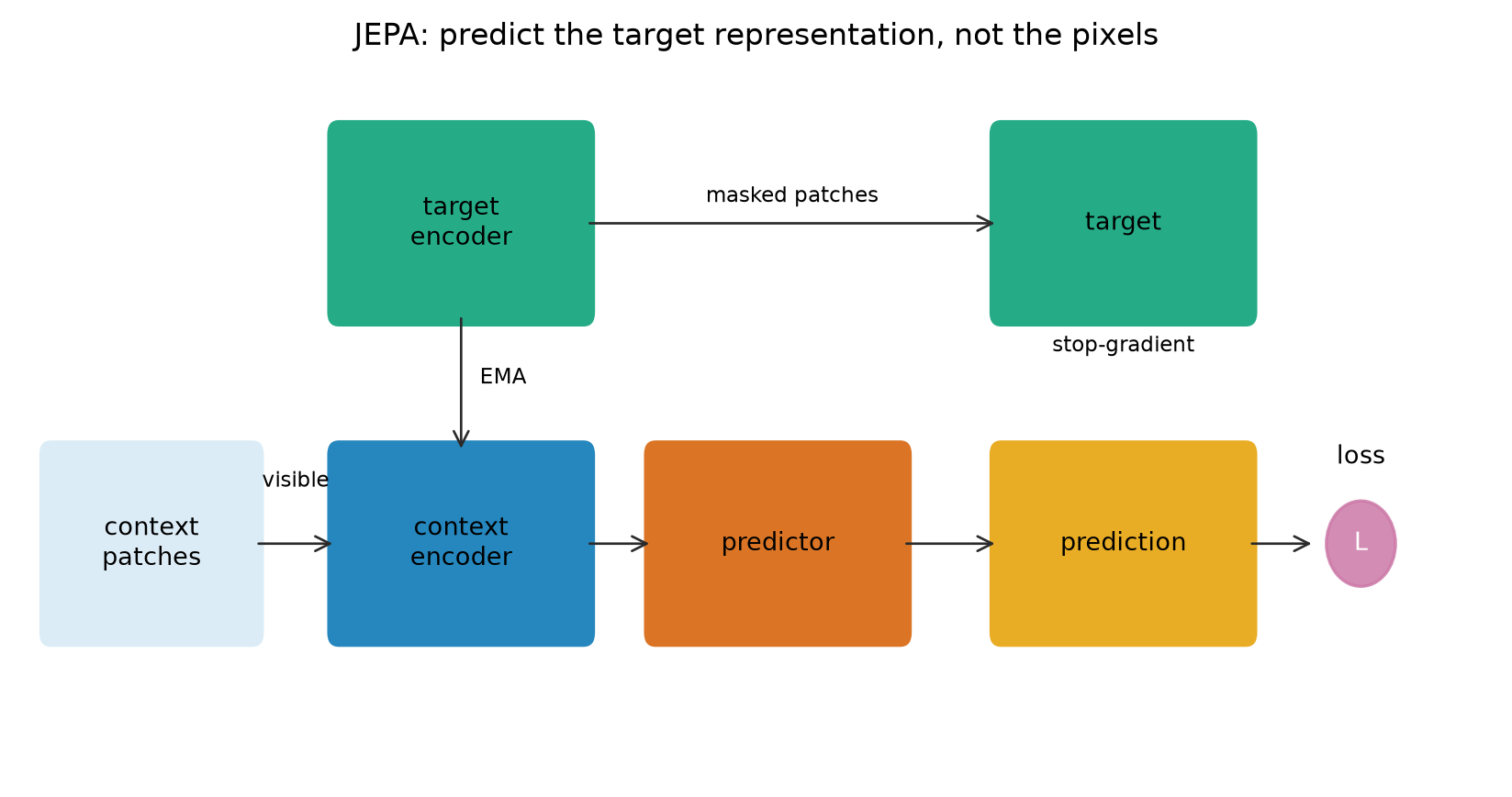
这张图里有五个零件。把它们分清,后面所有公式都只是给这五样东西写名字。
There are five parts in the figure. Keep them apart and every later equation is just naming these five things.
| 零件 / Part | 做什么 / What it does | 本文哪里 / Where here |
|---|---|---|
| 上下文编码器 / context encoder | 只看可见部分,输出可见 token / sees only visible patches, outputs visible tokens | 第 19 节 |
| 目标编码器 / target encoder | 看完整输入,输出预测目标;参数不反传 / sees the full input, produces targets; no gradient | 第 7、21 节 |
| 预测器 / predictor | 从可见 token 推断被遮位置的编码 / infers masked codes from visible tokens | 第 20 节 |
| 掩码与位置 / mask and positions | 决定”预测哪里”和”从哪里看” / decides what to predict and from where | 第 20 节 |
| 损失与 stop-gradient | 在表征空间比较,并切断目标侧梯度 / compares in representation space and cuts the target’s gradient | 第 12、21 节 |
English: the same five parts, one row each; the third column points to the section that implements it.
这里要先拆掉一个常见误解:JEPA 不是一种网络结构,而是一套训练目标加一个结构模板。 两个编码器可以是 ViT,也可以是卷积网络或 MLP;预测器可深可浅。真正定义 JEPA 的,是”预测表征、不预测观测”这一条目标函数,以及为了防止目标跟着预测一起移动而加的不对称性。
One common misunderstanding has to be removed first: JEPA is not a network architecture but an objective plus a structural template. The two encoders can be ViTs, convnets or MLPs; the predictor can be deep or shallow. What defines JEPA is the objective — predict representations, not observations — together with the asymmetry that stops the target from moving along with the prediction.
3. 基础概念:潜空间 / Latent space
一张 32×32 的彩色图片有 \(32\times32\times3=3072\) 个数值。把这 3072 个数看成一个点,它住在一个 3072 维的空间里。可是自然图像并不会均匀填满这个空间:随机抽 3072 个数,得到的几乎一定是电视雪花;能被称为”一只三角形”的点,只落在一个薄得多的曲面上。这个曲面常被叫作数据流形(data manifold)。
A 32×32 colour image has \(32\times32\times3=3072\) numbers. Treat those numbers as coordinates and the image is a point in a 3072-dimensional space. Natural images do not fill that space: draw 3072 numbers at random and you almost surely get television snow; the points we would call “a triangle” lie on a much thinner surface. That surface is usually called the data manifold.
潜空间(latent space)就是用来给这个流形重新编号的低维坐标系。编码器 \(f_\theta:\mathbb{R}^{3072}\to\mathbb{R}^{96}\) 把每个图像点送到一个 96 维向量;这个向量叫表征(representation)或嵌入(embedding),它的坐标就是”潜变量”。本文的玩具模型用 96 维,真实模型常用 768 到 4096 维——维度仍然远小于像素数,但比”三五种因素”高得多。
A latent space is a low-dimensional coordinate system that re-labels that manifold. An encoder \(f_\theta:\mathbb{R}^{3072}\to\mathbb{R}^{96}\) sends each image to a 96-dimensional vector; that vector is a representation or embedding, and its coordinates are the latent variables. The toy model here uses 96 dimensions; real models use 768 to 4096 — still far below the pixel count, but far above “three or five factors”.
必须强调:潜空间没有天然语义。 第 5 维不一定是”颜色”,第 17 维不一定是”位置”;坐标轴可以任意旋转、拉伸,只要损失不变。说”两个图像在潜空间里很近”,意思只是”在这个被训练出来的坐标系里,它们的向量夹角小或距离短”。这个距离是否对应人类理解的相似,完全取决于训练信号。把潜空间想成一张地图:地图上两点近,可能因为真的近,也可能因为绘图者把两个城市画在了一起。
One warning matters: a latent space has no intrinsic semantics. Dimension 5 is not necessarily “colour” and dimension 17 is not “position”; the axes can be rotated and stretched arbitrarily without changing the loss. Saying “two images are close in latent space” only means “in this trained coordinate system their vectors have a small angle or distance”. Whether that distance matches human similarity depends entirely on the training signal. Think of a map: two dots can be close because the places are close, or because the cartographer drew them that way.
JEPA 的特殊之处在于:潜空间不只是编码器的副产品,而是被预测的对象。预测器输出的是一段潜向量,损失也在这段潜向量上计算。所以潜空间的几何不是”顺便形成的”,而是目标函数直接塑造的——这既是它的力量,也是它坍塌的根源。
What is special about JEPA is that the latent space is not a by-product of the encoder but the object being predicted. The predictor outputs a latent vector and the loss is computed on it. The geometry of that space is therefore shaped directly by the objective — which is both its power and the root of its collapse risk.
4. 基础概念:自监督学习 / Self-supervised learning
监督学习需要标签:给图片,给人标的”三角形”,最小化交叉熵。无监督学习没有标签,通常指聚类、降维、密度估计。自监督学习(self-supervised learning, SSL)介于两者之间:没有人工标签,但可以从数据本身构造出预测目标。这个被构造出来的任务叫预训练任务(pretext task)。
Supervised learning needs labels: an image, a human-provided “triangle”, minimise cross-entropy. Unsupervised learning has no labels and usually means clustering, dimensionality reduction or density estimation. Self-supervised learning (SSL) sits between them: no human labels, but a prediction target constructed from the data itself. That constructed task is called a pretext task.
常见的 pretext task 有四类。语言模型猜下一个词;MAE 猜被遮住的像素;SimCLR 判断两张增强图是否来自同一张原图;JEPA 猜被遮区域的编码。这四类都可以写成”给一部分信息,预测另一部分信息”,区别在于预测什么、以及怎么防止模型作弊。
There are four common families. A language model guesses the next word; MAE guesses masked pixels; SimCLR decides whether two augmented views come from the same image; JEPA guesses the code of a masked region. All four can be written as “given part of the information, predict another part”; they differ in what is predicted and in how cheating is prevented.
| 家族 / Family | 预测什么 / Predicts | 防作弊手段 / Anti-cheat | 代表 / Examples |
|---|---|---|---|
| 生成式 / generative | 像素或词 / pixels or words | 目标固定,无法一起漂移 / target is fixed | MAE、扩散、GPT |
| 对比式 / contrastive | 正负样本关系 / positive vs negative | 负样本把不同样本推开 / negatives repel | SimCLR、MoCo |
| 联合嵌入非对比 / joint-embedding | 另一视角的编码 / code of another view | 不对称结构、EMA、正则 / asymmetry | BYOL、DINO、JEPA |
| 预测式自回归 / autoregressive | 下一 token / next token | 目标固定 / target is fixed | GPT、Llama |
English: one row per family; the third column is the mechanism that prevents the trivial constant solution.
三个词会在后文反复出现:预训练(在大数据上先学一个通用编码器)、微调(在下游任务上更新全部参数)、冻结(不动编码器,只训练一个小分类头)。本文所有比较都在”冻结 + 线性探针”的设置下进行,因为这样测的是表征本身,而不是某个任务上的拟合能力。
Three terms recur later: pre-training (learn a general encoder on large data), fine-tuning (update all parameters on a downstream task), and frozen (leave the encoder untouched and train only a small head). Every comparison here uses “frozen encoder + linear probe”, because that measures the representation rather than the fitting capacity of a task-specific head.
5. 基础概念:token、patch 与 Transformer / Tokens, patches and Transformers
Transformer 最初处理词序列。图像不是序列,所以 ViT(Vision Transformer)先把图像切成固定大小的方块:32×32 的图、8×8 的 patch,得到 \(4\times4=16\) 个 patch。每个 patch 有 \(3\times8\times8=192\) 个像素值,经过一个线性层或卷积变成 96 维向量。这个向量就叫一个 token。
Transformers were built for word sequences. Images are not sequences, so a ViT (Vision Transformer) first cuts the image into fixed-size squares: a 32×32 image with 8×8 patches gives \(4\times4=16\) patches. Each patch holds \(3\times8\times8=192\) pixel values and is mapped by a linear layer or convolution to a 96-dimensional vector. That vector is a token.
除了 patch token,还有两个小零件。位置编码(positional embedding)告诉模型”这个 token 原来在左上还是右下”,否则打乱顺序模型也分不出来。CLS token 是一个可学习的向量,被拼在序列最前面,经过若干层后它的输出常被当作整张图的摘要。自注意力(self-attention)是每一层里的混合操作:每个 token 用自己与别人的相似度算出一组权重,再把别人的信息加权求和取回来。一句话:token 之间互相看,看的权重由内容决定。
Besides patch tokens there are two small parts. A positional embedding tells the model whether a token came from the upper left or the lower right; without it, shuffling the tokens would be invisible. A CLS token is a learned vector prepended to the sequence whose output is often used as a summary of the whole image. Self-attention is the mixing operation in each layer: every token computes weights from its similarity to the others and takes a weighted sum of their information. In one sentence: tokens look at each other, and the weights depend on content.
现在可以回答一个常被问错的问题:JEPA 和 Transformer 是什么关系? 它们是两个层面的东西。Transformer 是躯干(把 token 混合起来的函数 approximator),JEPA 是训练目标(让躯干学什么)。I-JEPA 用的是 ViT,所以人们常把两者混在一起说;但把躯干换成卷积网络,JEPA 仍然成立;把目标换成下一 token 预测,Transformer 也仍然是 Transformer。LLM 是”Transformer + 自回归目标”,I-JEPA 是”Transformer + 联合嵌入预测目标”。
This answers a question that is often put wrongly: how are JEPA and Transformers related? They live on different levels. A Transformer is a body (a function approximator that mixes tokens); JEPA is an objective (what the body is trained to do). I-JEPA uses a ViT, which is why the two get conflated; but swap the body for a convnet and JEPA still stands, and swap the objective for next-token prediction and the Transformer is still a Transformer. An LLM is “Transformer + autoregressive objective”; I-JEPA is “Transformer + joint-embedding predictive objective”.
6. 基础概念:联合嵌入与坍塌 / Joint embedding and collapse
联合嵌入(joint embedding)指把两个相关的东西映射进同一个空间,再让它们的向量靠近。两个东西可以是同一张图的两个增强版本、一段视频的相邻两帧、一张图与被遮住的另一块。损失通常就是均方误差或余弦距离。
Joint embedding means mapping two related things into one space and pulling their vectors together. The two things can be two augmentations of an image, two adjacent video frames, or an image and one of its masked blocks. The loss is usually mean squared error or cosine distance.
如果只做这件事,会得到一个平凡解:把所有输入都映射成同一个向量。 这样任何一对的距离都是 0,损失完美。这叫完全坍塌(complete collapse)。还有一种较轻的维度坍塌(dimensional collapse):输出没有缩成一个点,但只落在一个低维子空间里,很多方向完全没有被使用。第三种最隐蔽,本文叫有效坍塌(effective collapse):向量看起来散布在各处,秩也不低,但尺度极小、方向主要是噪声,下游分类器拿不到信息。
Do only that and you get a trivial solution: map every input to the same vector. Every pair then has distance zero and the loss is perfect. That is complete collapse. A milder version is dimensional collapse: outputs are not a single point but lie in a low-dimensional subspace, leaving many directions unused. A third and subtler version, called effective collapse here, is when vectors appear spread out and the rank is not low, but their scale is tiny and their directions are mostly noise, so a downstream classifier gets nothing.
不同家族用不同办法避免这件事。生成式方法的目标是固定像素,像素不会为了迎合预测而移动,所以不会坍塌(但会模糊)。对比式方法用负样本把不同图像推开,常数解会被负样本惩罚。JEPA 的目标是另一个编码器的输出,这个输出会动;如果没有约束,两个编码器可以合谋把目标搬到预测旁边。这就是为什么 JEPA 必须额外引入不对称性。
Different families avoid this differently. Generative methods predict fixed pixels, which cannot move to meet the prediction, so they do not collapse (they blur instead). Contrastive methods use negatives to push different images apart, and a constant solution is punished by them. JEPA predicts the output of another encoder, which can move; without a constraint, the two encoders can collude and move the target next to the prediction. That is why JEPA must add asymmetry.
检测坍塌不能只看一个数。特征标准差(feature std)看每个维度是否有起伏;有效秩(effective rank)看奇异值分布是否铺开;平均余弦(mean cosine)看随机两点的方向是否几乎相同;线性探针看这些起伏是否线性可分。本文四个都报,因为它们的失效方式不同——第 24 节会看到一个”秩很高但标准差接近零”的例子,只看秩会得出完全相反的结论。
No single number detects collapse. Feature standard deviation asks whether each dimension varies; effective rank asks whether the singular-value spectrum is spread out; mean cosine asks whether two random points point in almost the same direction; a linear probe asks whether the variation is linearly decodable. All four are reported here because they fail differently — Section 24 shows a case with high rank and near-zero standard deviation, where rank alone gives the opposite conclusion.
7. 基础概念:stop-gradient、EMA 与正则 / Stop-gradient, EMA and regularisation
stop-gradient(记为 \(\mathrm{sg}\))是一个只在前向传播时存在的恒等函数:前向时 \(\mathrm{sg}(u)=u\),反向时把梯度置零。用在目标侧,意思是”目标可以随便算,但不要为了降低损失而修改目标”。数学上它把损失对目标编码器的梯度从计算图里切断,只有上下文编码器和预测器收到更新。
Stop-gradient (written \(\mathrm{sg}\)) is an identity that exists only in the forward pass: \(\mathrm{sg}(u)=u\) forward, zero gradient backward. Applied to the target side it means “compute the target however you like, but do not change it in order to lower the loss”. Mathematically it cuts the target encoder out of the gradient graph; only the context encoder and the predictor are updated.
EMA(exponential moving average,指数滑动平均)解决另一个问题:即使目标侧不反传,如果目标编码器就是上下文编码器的同一个副本,它仍然会每一步跟着变。EMA 让目标编码器变成上下文编码器的滞后副本:
EMA (exponential moving average) solves a different problem: even with no gradient on the target side, if the target encoder is the same copy as the context encoder it still changes at every step. EMA makes the target a lagged copy of the context encoder:
\[ \bar\theta \leftarrow m\,\bar\theta + (1-m)\,\theta . \]
\(m\) 越接近 1,目标越滞后。\(m=0.99\) 的时间常数约为 \(1/(1-m)=100\) 步,\(m=0.999\) 约为 1000 步。直观上,目标是一个”过去若干步编码器的滑动平均”,它不会跟着当前批次立刻漂移,于是预测任务保持了一定的稳定性。
The closer \(m\) is to 1, the more lagged the target. With \(m=0.99\) the time constant is about \(1/(1-m)=100\) steps; with \(m=0.999\) it is about 1000. Intuitively the target is a moving average of the encoder over the recent past, so it does not drift with the current batch and the prediction task stays relatively stable.
第三类办法是显式正则。VICReg 对方差和协方差各加一项:每个维度的标准差不能低于 1,不同维度之间的协方差要接近 0。前者防止所有维度缩成一个点,后者防止维度之间重复。LeJEPA 的 SIGReg 走得更远:用随机投影把嵌入投到若干一维方向,再要求这些投影的分布接近标准正态——一个各向同性的高斯既不会坍塌,也不会把信息挤在少数方向上。
The third family is explicit regularisation. VICReg adds a variance term (the standard deviation of each dimension should not fall below 1) and a covariance term (different dimensions should be uncorrelated). The first stops all dimensions shrinking to a point, the second stops redundancy. LeJEPA’s SIGReg goes further: random projections map the embedding to several one-dimensional directions, and each projected distribution is pushed toward a standard normal — an isotropic Gaussian neither collapses nor squeezes information into a few directions.
| 稳定器 / Stabiliser | 机制 / Mechanism | 防什么 / Prevents | 代价 / Cost |
|---|---|---|---|
| stop-gradient | 切断目标侧梯度 / cut target gradient | 目标被拉向预测 / target dragged to prediction | 无额外计算 / free |
| EMA | 目标编码器滞后更新 / lagged target | 目标快速漂移 / fast target drift | 多一份参数 / extra copy |
| 方差-协方差正则 / VICReg | 方差下限 + 去相关 / variance floor + decorrelation | 完全与维度坍塌 / complete and dimensional collapse | 一个超参数 / one weight |
| SIGReg | 投影分布逼近高斯 / projected Gaussianity | 坍塌且保持各向同性 / collapse and anisotropy | 投影与检验 / projections and test |
English: four stabilisers, what each prevents, and what it costs.
8. 基础概念:线性探针与”表征好不好” / Linear probes and representation quality
训练完一个编码器,怎么知道它学到的表征好不好?最常用的办法是线性探针(linear probe):冻结编码器,把所有输入过一遍得到特征,再在特征上训练一个线性分类器(本文用逻辑回归)。如果线性分类器就能把形状分对,说明形状信息在表征里是线性可读的。
How do we know whether a trained encoder learned a good representation? The usual answer is a linear probe: freeze the encoder, run all inputs through it to get features, then fit a linear classifier on the features (logistic regression here). If a linear classifier can separate shapes, shape information is linearly readable in the representation.
为什么强调”线性”?因为非线性分类器太强,几乎什么表征都能拟合,测出来的就不是表征的质量,而是探针的容量。把探针限制成线性,等于问一个很保守的问题:信息有没有被摆到容易取用的位置上? 这个问题不完美,但可比性强。
Why insist on “linear”? A non-linear classifier is strong enough to fit almost any representation, so the number would measure the probe rather than the representation. Restricting to linear asks a conservative question: has the information been placed somewhere easy to read? The question is imperfect but comparable across models.
探针有三个陷阱,本文都会遇到。第一,标准化会掩盖坍塌:如果特征尺度极小,StandardScaler 会把噪声放大到单位方差,线性探针的准确率会虚高;第 24 节的 0.5625 与 0.369 就是这个差别。第二,线性可读不等于模型在用:表征里可能有颜色信息,但模型做预测时并不依赖它。第三,探针准确率不是下游性能:检测、分割、控制任务需要的几何性质与分类不同。
Three traps appear in this article. First, standardisation can hide collapse: if feature scale is tiny, StandardScaler rescales noise to unit variance and the probe looks better than it is; the 0.5625 versus 0.369 in Section 24 is exactly this gap. Second, linear readability is not use: colour may be present in the representation without the model relying on it. Third, probe accuracy is not downstream performance: detection, segmentation and control need different geometry from classification.
本文还报一个回归指标:用岭回归从特征预测目标的中心坐标,报告 position RMSE(均方根误差),单位是图像边长的比例。它比分类更细,能看出表征是否保留了连续的空间信息。
One regression metric is also reported: ridge regression predicts the object’s centre from the features, and position RMSE (root mean squared error) is reported in units of image side length. It is finer than classification and shows whether continuous spatial information survives.
9. JEPA 与下一个 token 预测 / JEPA versus next-token prediction
大语言模型的目标是 \(p(x_t\mid x_{<t})\):给定前文,预测下一个离散 token。损失是交叉熵,输出是词表上的分布,采样后接回输入,如此循环。这个目标极其成功,因为它把”理解”压缩成了”能否猜对下一个词”,而语言的下一个词确实携带大量语义。
A large language model’s objective is \(p(x_t\mid x_{<t})\): given the prefix, predict the next discrete token. The loss is cross-entropy, the output is a distribution over the vocabulary, and sampling feeds back into the input. The objective is extraordinarily successful because it compresses “understanding” into “can you guess the next word”, and in language the next word really does carry semantics.
JEPA 的目标不是 token,而是连续表征:\(g_\phi(f_\theta(x))\approx f_{\bar\theta}(y)\)。它没有词表,没有 softmax,也不需要把目标解码回可读形式。它不要求模型说清”下一个像素/词是什么”,只要求它在表征空间里落到正确的位置。对于视频这类细节极其丰富、未来本质多义的输入,这一点很关键:树叶的每一片抖动都无法预测,硬要预测只会得到模糊的平均。
JEPA’s target is not a token but a continuous representation: \(g_\phi(f_\theta(x))\approx f_{\bar\theta}(y)\). There is no vocabulary, no softmax, and no need to decode the target back into a readable form. The model is not asked to say what the next pixel or word is, only to land in the right place in representation space. For video, where detail is enormous and the future genuinely multi-valued, this matters: no one can predict every leaf, and forcing it yields a blurry average.
| 维度 / Dimension | 下一 token 预测 / next-token | JEPA |
|---|---|---|
| 预测空间 / target space | 离散词表 / discrete vocabulary | 连续表征 / continuous representation |
| 损失 / loss | 交叉熵 / cross-entropy | L2 或 smooth L1 |
| 解码器 / decoder | 必需(softmax)/ required | 不需要 / none |
| 坍塌风险 / collapse risk | 低(目标固定)/ low | 高(目标可动)/ high |
| 不确定性 / uncertainty | 词表上的分布 / distribution | 靠丢弃细节或隐变量 / drop detail or latent |
| 典型用途 / typical use | 语言、代码 / language, code | 视觉、视频、控制 / vision, video, control |
English: the same comparison, one row per dimension.
两者不是互斥的。LLM-JEPA 就是在语言模型上同时保留下一 token 损失和 JEPA 损失:前者保证能生成,后者把两个视角的中间表征拉近。第 34 节会回到这个例子。
The two are not exclusive. LLM-JEPA keeps both the next-token loss and a JEPA loss on a language model: the first preserves generation, the second pulls the intermediate representations of two views together. Section 34 returns to this.
10. 目标函数的四象限 / A map of objectives
把现有方法放在两个坐标轴上,可以看到它们各自的取舍。横轴是预测目标:最左边是原始观测(像素),最右边是学出来的表征。纵轴是不变性:最下面是”没有显式不变性”,最上面是”通过增强或结构学出来的不变性”。这张图的坐标是定性判断,不是测量值。
Put existing methods on two axes and their trade-offs become visible. The horizontal axis is the prediction target: raw observation (pixels) on the left, learned representation on the right. The vertical axis is invariance: none at the bottom, invariance learned through augmentations or architecture at the top. The coordinates are qualitative, not measured.
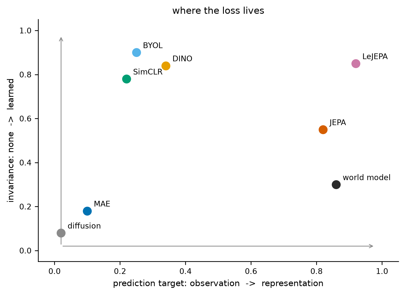
这张图解释了为什么 JEPA 不是”又一个自监督方法”,而是一个位置:它把预测目标推到最右,同时把不变性交给目标编码器和掩码策略去学,而不是手工设计增强。代价是右上方那片区域最难稳定——目标越抽象,越容易坍塌。这也解释了为什么 JEPA 的论文里有大量篇幅在讲掩码、EMA 和正则,而不是讲网络结构。
The figure explains why JEPA is not “another self-supervised method” but a position: it pushes the prediction target to the far right and delegates invariance to the target encoder and the masking strategy instead of hand-designed augmentations. The price is that the upper-right region is the hardest to stabilise — the more abstract the target, the easier it collapses. This is also why JEPA papers spend pages on masking, EMA and regularisation rather than on architecture.
11. 从 2022 到 2026:一条时间线 / A timeline, 2022–2026
JEPA 这个词来自 LeCun 2022 年 6 月的立场文章《A Path Towards Autonomous Machine Intelligence》。文章不是一个模型,而是一张蓝图:感知、世界模型、代价模块、配置器,JEPA 是其中负责”在表征空间预测”的那块。2023 年的 I-JEPA 第一次把它落到图像上,2024 年的 V-JEPA 把它推到视频,2025 年的 V-JEPA 2 把它接到机器人规划,同年 LeJEPA 试图用理论去掉启发式,2026 年出现了多模态与跨领域的扩展。
The word JEPA comes from LeCun’s June 2022 position paper, A Path Towards Autonomous Machine Intelligence. The paper is not a model but a blueprint — perception, world model, cost module, configurator — and JEPA is the part responsible for “prediction in representation space”. I-JEPA (2023) put it on images, V-JEPA (2024) on video, V-JEPA 2 (2025) on robot planning; LeJEPA (2025) tried to replace heuristics with theory, and 2026 brought multimodal and cross-domain extensions.
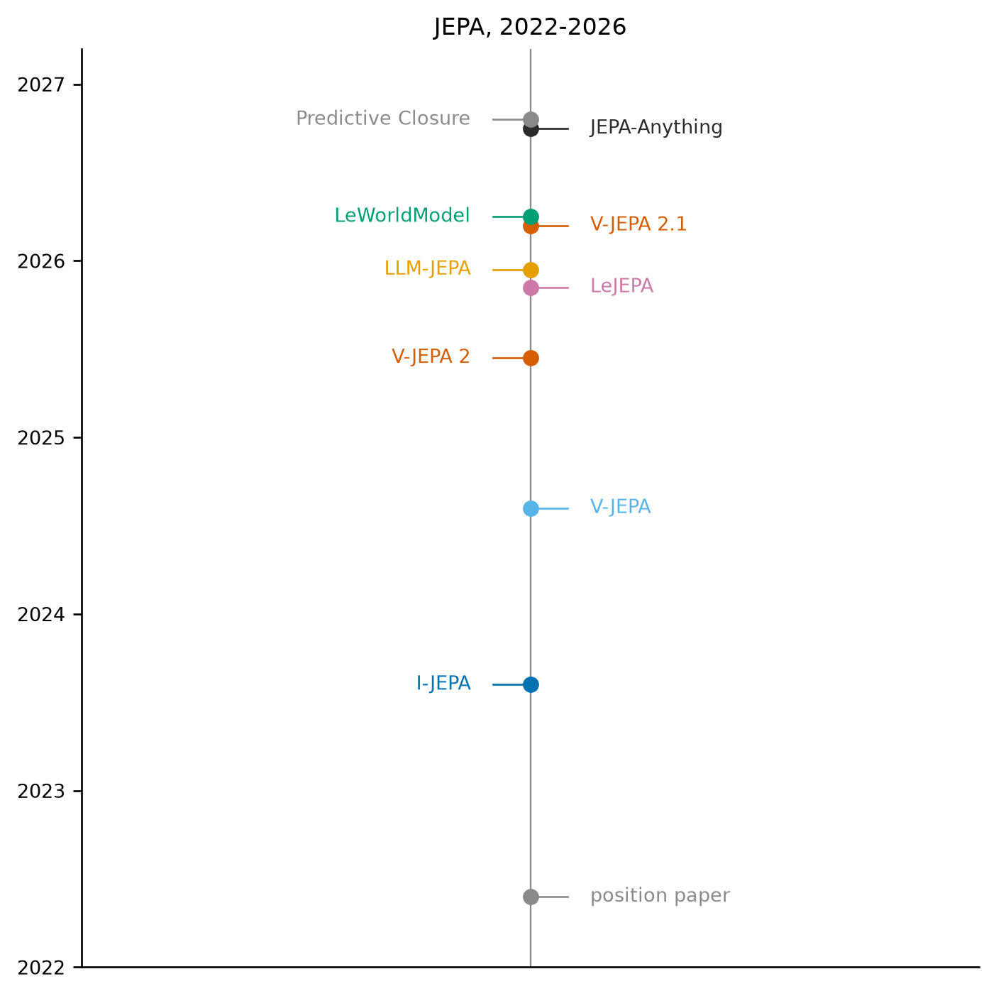
这条线有三个趋势。第一,从图像到视频再到动作:预测的目标越来越接近”世界如何变化”,而不只是”这张图里有什么”。第二,从启发式到理论:早期的 stop-gradient 和 EMA 是工程技巧,LeJEPA 与 Predictive Closure 试图说清它们为什么有效、什么时候不需要。第三,从单领域到多领域:JEPA-Anything 把同一套目标套到七个数据域上。三个趋势都还没有收敛,下面的实验只能触及第一条的一小段。
Three trends run through it. First, from images to video to action: the prediction target moves toward “how the world changes”, not just “what is in this image”. Second, from heuristics to theory: early stop-gradient and EMA were engineering tricks; LeJEPA and Predictive Closure try to explain why they work and when they are unnecessary. Third, from one domain to many: JEPA-Anything applies one objective across seven data domains. None of the three has converged, and the experiments below touch only a small part of the first.
12. 形式化定义 / A formal definition
设观测 \(x\in\mathcal{X}\),预测目标 \(y\in\mathcal{Y}\),两者来自同一个数据分布。JEPA 有三个可学习或半可学习的部件:上下文编码器 \(f_\theta\)、目标编码器 \(f_{\bar\theta}\)、预测器 \(g_\phi\)。训练目标是
Let \(x\in\mathcal{X}\) be the observation and \(y\in\mathcal{Y}\) the prediction target, both drawn from the same data distribution. JEPA has three learnable or semi-learnable parts: a context encoder \(f_\theta\), a target encoder \(f_{\bar\theta}\), and a predictor \(g_\phi\). The training objective is
\[ \mathcal{L}(\theta,\phi) = \mathbb{E}_{(x,y)\sim p_{\text{data}}} \left[ \left\| g_\phi\big(f_\theta(x),\,c\big) - \mathrm{sg}\big(f_{\bar\theta}(y)\big) \right\|^2 \right], \qquad \bar\theta \leftarrow m\,\bar\theta + (1-m)\,\theta . \]
逐项解释。\(f_\theta(x)\) 是可见部分的编码;\(c\) 是条件信息,在图像里是”要预测哪些位置”,在世界模型里是动作;\(g_\phi\) 输出预测的表征;\(f_{\bar\theta}(y)\) 是目标编码器对完整目标的编码;\(\mathrm{sg}\) 切断目标侧梯度;最后一行是 EMA 更新,\(m\) 是动量。注意 \(\bar\theta\) 不出现在损失对参数的梯度里,它只通过 EMA 缓慢跟随 \(\theta\)。
Term by term: \(f_\theta(x)\) encodes the visible part; \(c\) is conditioning information — which positions to predict for images, the action for a world model; \(g_\phi\) outputs the predicted representation; \(f_{\bar\theta}(y)\) encodes the full target; \(\mathrm{sg}\) cuts the target-side gradient; the last line is the EMA update with momentum \(m\). Note that \(\bar\theta\) never appears in the gradient of the loss with respect to parameters; it only follows \(\theta\) slowly through EMA.
三个实例化值得记住。I-JEPA:\(x\) 是一个上下文块,\(y\) 是若干目标块,\(c\) 是目标块的位置,掩码是多块而非单块。V-JEPA:\(x,y\) 是视频中不同时间或空间区域,掩码是时空管(tube)。世界模型:\(x\) 是当前帧,\(y\) 是下一帧,\(c\) 是动作 \(a_t\),预测器变成动作条件预测器。三者的损失形式完全一样,变的只是”什么算目标”和”条件是什么”。
Three instantiations are worth remembering. I-JEPA: \(x\) is one context block, \(y\) several target blocks, \(c\) their positions, and the mask is multi-block rather than a single rectangle. V-JEPA: \(x\) and \(y\) are spatio-temporal regions, and masks are tubes. World model: \(x\) is the current frame, \(y\) the next frame, \(c\) the action \(a_t\), and the predictor becomes action-conditioned. The loss is identical; only “what counts as a target” and “what the condition is” change.
13. 为什么在表征空间预测 / Why predict in representation space
先看像素空间里发生了什么。给定上下文 \(x\),用均方误差训练一个预测器 \(h\),最优解是条件均值:
Start with what happens in pixel space. Given a context \(x\), train a predictor \(h\) with squared error; the optimum is the conditional mean:
\[ h^\star(x)=\arg\min_{c}\ \mathbb{E}\big[\|c-y\|^2\mid x\big]=\mathbb{E}[y\mid x]. \]
如果同一个 \(x\) 对应多个合理的未来——球可能向左也可能向右,云可能这样飘也可能那样飘——条件均值就是这些未来的平均。平均一张”向左的球”和一张”向右的球”,得到的是一团模糊的影子。这不是模型不够大,而是目标函数本身要求的:平方误差下,说真话的最优方式就是报平均值。
If the same \(x\) admits several plausible futures — the ball may go left or right, the cloud may drift this way or that — the conditional mean is the average of those futures. Averaging a ball going left and a ball going right gives a blurry ghost. This is not a capacity problem; the objective demands it: under squared error, the optimal honest answer is the mean.
把目标换成 \(f_{\bar\theta}(y)\) 会改变这个回归。如果目标编码器已经丢弃了不可预测的细节,只保留”球在哪、往哪走”这类可预测的量,那么条件均值在这个空间里可以是清晰的。信息瓶颈(information bottleneck)给了同一件事一个信息论的写法:在最小化 \(I(z;x)\) 的同时最大化 \(I(z;y)\),即”编码尽量少,但对目标尽量有用”。JEPA 没有显式写这个约束,但目标编码器加预测器瓶颈在近似它。
Replacing the target with \(f_{\bar\theta}(y)\) changes the regression. If the target encoder has already discarded unpredictable detail and kept predictable quantities such as where the ball is and where it is heading, the conditional mean in that space can be sharp. The information bottleneck gives the same idea an information-theoretic form: minimise \(I(z;x)\) while maximising \(I(z;y)\) — “encode as little as possible, but as much as is useful about the target”. JEPA does not impose this constraint explicitly, but a target encoder plus a narrow predictor approximates it.
代价是:目标编码器决定了什么算”可预测”,而它是学出来的。 如果它太粗,任务变得平凡,预测器随便猜都能中;如果它太细,任务退化成像素预测,模糊问题又回来。I-JEPA 的实验给出的经验是,目标块要足够大(才携带语义),上下文要空间分散(才提供足够信息)。这两个条件都不是网络结构决定的,而是掩码策略决定的——所以第 25 节会专门扫掩码比例。
The price: the target encoder decides what counts as predictable, and it is learned. Too coarse and the task is trivial, so the predictor can guess anything; too fine and the task degenerates into pixel prediction and blur returns. I-JEPA’s empirical lesson is that target blocks must be large enough to carry semantics and the context spatially distributed enough to be informative. Neither condition is set by the architecture; both are set by the masking strategy — which is why Section 25 sweeps the mask ratio.
14. 坍塌的数学 / The mathematics of collapse
先看最简单的情形:线性编码器 \(f(x)=Wx\),预测器取恒等,目标编码器与上下文编码器共享参数。损失是
Take the simplest case: a linear encoder \(f(x)=Wx\), an identity predictor, and a target encoder tied to the context encoder. The loss is
\[ \mathcal{L}(W)=\mathbb{E}\big[\|Wx-Wy\|^2\big]. \]
\(W=0\) 是一个全局最优解,损失为 0。更糟的是,这不是一个孤立的坏点:只要 \(W\) 的奇异值整体缩小,损失就单调下降。梯度下降会顺着这条下坡路走,把编码器推向”输出越来越小、方向越来越不重要”的区域。这就是为什么共享参数、没有 stop-gradient 的联合嵌入目标天然倾向于坍塌。
\(W=0\) is a global optimum with zero loss. Worse, it is not an isolated bad point: shrink every singular value of \(W\) and the loss decreases monotonically. Gradient descent follows that slope and pushes the encoder toward “smaller outputs, less important directions”. This is why a tied joint-embedding objective without stop-gradient is naturally attracted to collapse.
有效秩给”表征铺开了多少方向”一个数。把特征矩阵中心化,做奇异值分解,得到 \(\sigma_1\ge\sigma_2\ge\cdots\ge\sigma_d\ge0\)。令 \(p_i=\sigma_i/\sum_j\sigma_j\),则
Effective rank turns “how many directions are used” into a number. Centre the feature matrix, take its singular values \(\sigma_1\ge\sigma_2\ge\cdots\ge\sigma_d\ge0\), set \(p_i=\sigma_i/\sum_j\sigma_j\), and define
\[ H=-\sum_{i=1}^{d}p_i\log p_i, \qquad \mathrm{erank}=\exp(H). \]
它的范围是 \(1\) 到 \(d\):奇异值全集中在一个方向上时 \(H=0\)、\(\mathrm{erank}=1\);奇异值均匀铺开时 \(H=\log d\)、\(\mathrm{erank}=d\)。它衡量的是谱的形状,不是幅度。这一点极重要:把所有特征乘以 \(10^{-6}\),有效秩一点不变。
Its range is \(1\) to \(d\): if all singular values sit on one direction, \(H=0\) and \(\mathrm{erank}=1\); if they are uniform, \(H=\log d\) and \(\mathrm{erank}=d\). It measures the shape of the spectrum, not its magnitude. That matters enormously: multiply every feature by \(10^{-6}\) and the effective rank does not change.
与之互补的是尺度类指标。第 \(j\) 维的标准差 \(\mathrm{std}_j=\sqrt{\mathrm{Var}(f_j)}\),取平均得到 feature std;随机抽两点算余弦相似度,取平均得到 mean cosine。前者接近 0 表示所有点挤在一起,后者接近 1 表示所有方向几乎相同。第 24 节会看到:联合训练那一组的有效秩是 40.09,看起来”很铺开”,但 feature std 只有 0.0035——谱的形状很宽,幅度却几乎为零。只看秩会把这种状态误判为健康。
The complementary metrics are scale-sensitive. The standard deviation of dimension \(j\) is \(\mathrm{std}_j=\sqrt{\mathrm{Var}(f_j)}\); averaging gives feature std. The mean cosine between random pairs gives mean cosine: near 0 means all points are piled together, near 1 means all directions coincide. Section 24 shows a joint-training run with effective rank 40.09 — apparently “spread out” — but feature std only 0.0035. The spectrum is wide in shape and almost zero in magnitude. Rank alone would call this healthy.
15. 稳定器的数学 / The mathematics of the stabilisers
stop-gradient 的作用可以直接从梯度看出来。损失对上下文编码器参数的梯度是
The effect of stop-gradient is visible directly in the gradient. The gradient with respect to the context encoder is
\[ \frac{\partial\mathcal{L}}{\partial\theta} = 2\,\mathbb{E}\Big[ \big(g_\phi(f_\theta(x))-z_y\big)^{\top} \frac{\partial g_\phi}{\partial f_\theta} \frac{\partial f_\theta}{\partial\theta} \Big], \qquad z_y=\mathrm{sg}\big(f_{\bar\theta}(y)\big), \]
其中 \(z_y\) 被视为常数,\(\partial z_y/\partial\bar\theta\) 不进入这条链。目标是”回归到一个会慢慢移动的靶子”,这在形式上与强化学习里的自举(bootstrapping)很像:用当前估计构造目标,再向目标回归。区别是这里的靶子来自另一个编码器,而不是同一个值函数。
where \(z_y\) is treated as a constant and \(\partial z_y/\partial\bar\theta\) never enters the chain. The target is “regress onto a slowly moving target”, which formally resembles bootstrapping in reinforcement learning: build a target from a current estimate, then regress onto it. The difference is that the target here comes from a different encoder rather than from the same value function.
EMA 的闭式解说明它为什么”慢”:
The closed form of EMA shows why it is slow:
\[ \bar\theta_t=(1-m)\sum_{k=0}^{t-1}m^{k}\,\theta_{t-k}+m^{t}\,\bar\theta_0 . \]
权重按 \(m^k\) 衰减,等效窗口长度约为 \(1/(1-m)\)。\(m=0.99\) 时窗口约 100 步,\(m=0.999\) 时约 1000 步。窗口越长,目标越稳定,但也越滞后于当前编码器;如果训练分布变化快,滞后会变成负担。本文的玩具训练只有几百到一千步,所以 \(m=0.999\) 的窗口几乎覆盖全程,目标几乎是”初始编码器加一点点变化”——这也是第 24 节里它虽然方差大、探针却没变好的原因之一。
Weights decay as \(m^k\), so the effective window is about \(1/(1-m)\): roughly 100 steps at \(m=0.99\) and 1000 at \(m=0.999\). A longer window gives a more stable but more lagged target; if the data distribution moves fast, the lag becomes a liability. The toy runs here last only a few hundred to a thousand steps, so an \(m=0.999\) window covers almost the whole run — the target is nearly the initial encoder plus a small perturbation. That is part of why it shows larger variance without a better probe in Section 24.
显式正则写成损失项更直接。VICReg 的形式是
Explicit regularisation is easier to write as loss terms. VICReg uses
\[ \mathcal{L}_{\text{VICReg}} = \lambda\sum_{j}\max\big(0,\,1-\mathrm{std}_j\big) + \mu\sum_{i\ne j}C_{ij}^{2}, \qquad C=\frac{1}{n-1}Z^{\top}Z, \]
其中 \(Z\) 是中心化后的特征矩阵。第一项给每个维度设一个方差下限(低于 1 就罚),第二项惩罚不同维度之间的相关性。SIGReg 换了一个角度:抽若干随机单位向量 \(u_k\),要求 \(u_k^{\top}z\) 的分布接近 \(\mathcal{N}(0,1)\)。高斯分布是各向同性的、非退化的,所以这个约束同时反对坍塌与各向异性。要强调的是:这些约束保证的是非退化,不是语义;一个各向同性的高斯潜空间可以完全没有类别结构。
where \(Z\) is the centred feature matrix. The first term imposes a variance floor (penalty below 1), the second penalises correlation between dimensions. SIGReg takes another route: draw random unit vectors \(u_k\) and require \(u_k^{\top}z\) to be distributed like \(\mathcal{N}(0,1)\). A Gaussian is isotropic and non-degenerate, so the constraint opposes both collapse and anisotropy. The caveat: these constraints guarantee non-degeneracy, not semantics; an isotropic Gaussian latent space can have no class structure at all.
16. 能量视角 / An energy-based view
能量模型(energy-based model, EBM)用一个标量函数 \(E_\theta(x,y)\) 给”输入与输出是否相容”打分:相容时能量低,不相容时能量高。推理就是给定 \(x\) 求 \(y^\star=\arg\min_y E_\theta(x,y)\);训练则要压低真实配对的能量、抬高其他配对的能量。JEPA 的损失 \(\|g_\phi(f_\theta(x))-f_{\bar\theta}(y)\|^2\) 正是一个能量:预测表征与目标表征越远,能量越高。
An energy-based model (EBM) scores “how compatible are \(x\) and \(y\)” with a scalar \(E_\theta(x,y)\): low when compatible, high when not. Inference solves \(y^\star=\arg\min_y E_\theta(x,y)\); training lowers the energy of real pairs and raises it for others. JEPA’s loss \(\|g_\phi(f_\theta(x))-f_{\bar\theta}(y)\|^2\) is exactly an energy: the further the predicted representation from the target, the higher it is.
LeCun 的立场文章把这个能量放进一个更大的架构:感知模块(JEPA)产生状态的表征,世界模型预测下一个状态,代价模块给状态打分,配置器决定当前该做什么。规划就是在这个能量面上做优化——给定目标状态,搜索一串动作,使最终状态的能量最低。
LeCun’s position paper places this energy inside a larger architecture: a perception module (JEPA) produces state representations, a world model predicts the next state, a cost module scores states, and a configurator decides what to do. Planning is optimisation on that energy surface: given a goal state, search for an action sequence whose final state has the lowest energy.
这里必须加一句限定:“能量”是一种建模语言,不是概率保证。 JEPA 没有配分函数,没有归一化的似然,也没有校准过的置信度。把损失叫能量,能帮助我们把感知与规划放进同一个优化框架,但它不会自动给出”这个预测有多可信”。第 28 节的规划失败,某种意义上就是能量面形状不对:表征空间里的低能量点,不一定是物理上想要的状态。
One qualification is necessary: “energy” is a modelling language, not a probabilistic guarantee. JEPA has no partition function, no normalised likelihood and no calibrated confidence. Calling the loss an energy helps place perception and planning in one optimisation framework, but it does not say how trustworthy a prediction is. The planning failure in Section 28 is, in a sense, a wrong energy landscape: a low-energy point in representation space need not be the physically desired state.
17. 从预测到规划 / From prediction to planning
世界模型(world model)指的是一个能在内部模拟”如果这样做,接下来会怎样”的模型。Ha 与 Schmidhuber 在 2018 年的工作把它拆成两部分:一个把观测压成潜状态的编码器,一个在潜空间里预测下一状态的转移模型;规划在潜空间里做,不必生成每一帧像素。JEPA 的世界模型版本把转移模型换成动作条件的预测器:\(\hat z_{t+1}=P_\phi(\hat z_t,a_t)\)。
A world model is a model that can internally simulate “if I do this, what happens next”. Ha and Schmidhuber (2018) split it into an encoder that compresses observations into latent states and a transition model that predicts the next state in that latent space; planning happens in the latent space without generating every pixel. The JEPA version replaces the transition model with an action-conditioned predictor: \(\hat z_{t+1}=P_\phi(\hat z_t,a_t)\).
在潜空间里选动作,常用 CEM(cross-entropy method,交叉熵方法)。它的循环只有四步:
To choose actions in latent space, a common tool is the cross-entropy method (CEM). Its loop has four steps:
- 采样:从当前高斯分布 \(\mathcal{N}(\mu,\sigma^2)\) 抽 \(N\) 条长度为 \(H\) 的动作序列。
Sample \(N\) action sequences of length \(H\) from the current Gaussian \(\mathcal{N}(\mu,\sigma^2)\). - 评估:把每条序列喂进世界模型,滚出最终潜状态,算代价 \(\|\hat z_H-z_g\|^2\)。
Evaluate each sequence by rolling the world model forward and computing \(\|\hat z_H-z_g\|^2\). - 择优:保留代价最低的 \(k\) 条。
Keep the \(k\) sequences with the lowest cost. - 重估:用这 \(k\) 条的均值和标准差更新 \(\mu,\sigma\),回到第一步。
Refit \(\mu,\sigma\) on those \(k\) and repeat.
迭代若干轮后,取均值序列的第一个动作执行,然后在下一个时刻重新规划。这个”只执行第一步”的策略叫 MPC(model predictive control,模型预测控制),它用频繁重规划来抵消模型误差。
After a few iterations, execute the first action of the mean sequence and replan at the next step. Executing only the first action is model predictive control (MPC); frequent replanning compensates for model error.
潜空间规划的好处是便宜:一次前向传播作用在 96 维而不是 3072 维,\(N\times H\) 条候选也不需要解码成图像。LeWorldModel 报告过最高 48 倍的规划加速,条件相同的情况下,这个数量级是可信的。风险则在代价函数:潜空间里的欧氏距离不等于物理距离,也不等于任务成功。第 28 节会看到,这个风险在玩具环境里直接兑现成了失败。
Latent planning is cheap: one forward pass acts on 96 dimensions instead of 3072, and \(N\times H\) candidates never need decoding into images. LeWorldModel reports planning speed-ups of up to 48×; under the same conditions that order of magnitude is plausible. The risk sits in the cost function: Euclidean distance in latent space is neither physical distance nor task success. Section 28 shows this risk turning directly into failure in the toy environment.
18. 实验全景:数据、模型与协议 / The experimental setup
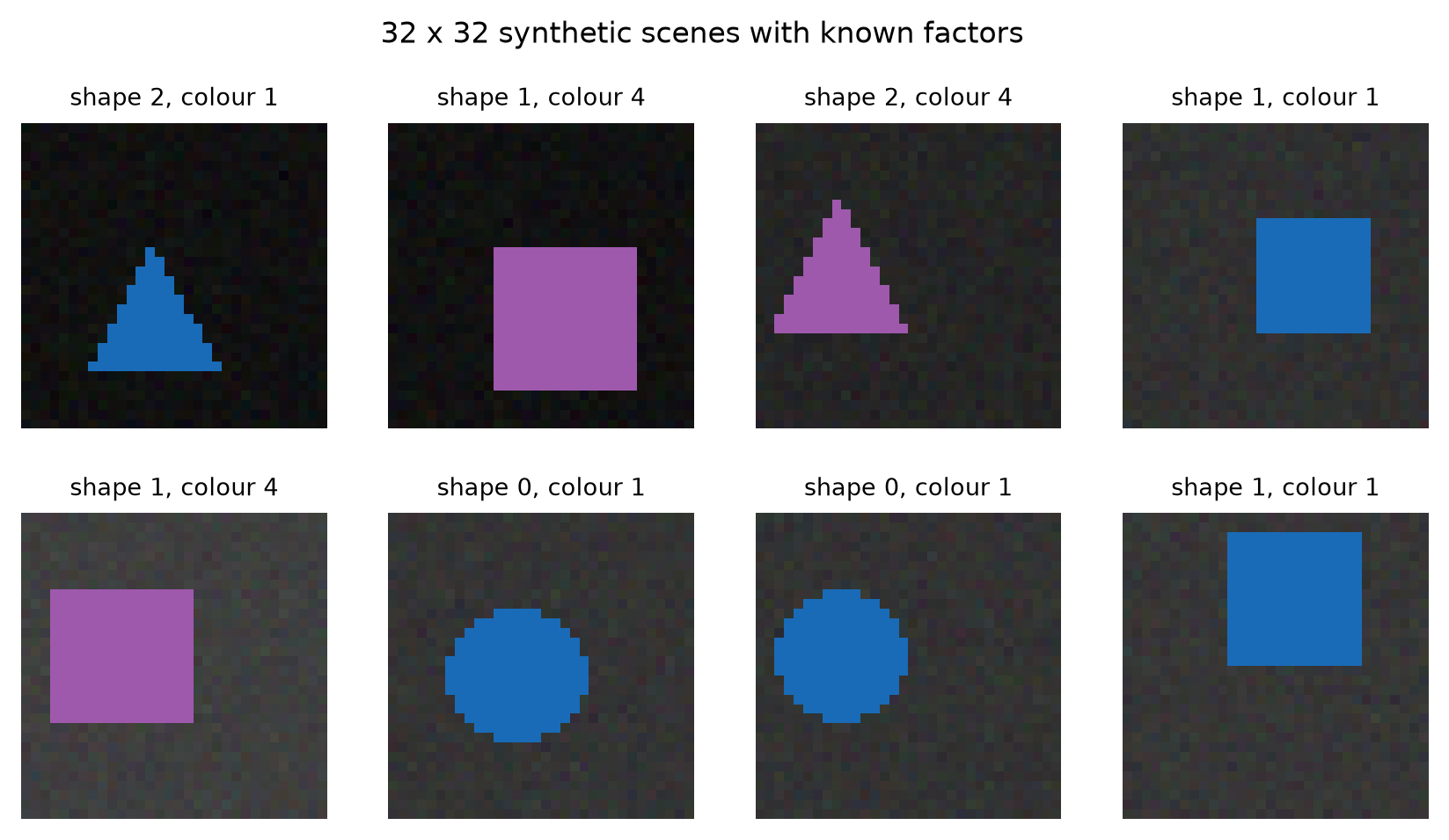
所有实验用两类合成数据。第一类是 32×32 的图形场景:形状有三种(圆、方、三角),颜色有五种,中心位置在 \([0.25,0.75]^2\) 内均匀采样,半径 0.14–0.22,背景亮度 0.05–0.25,另加标准差 0.015 的像素噪声。因为形状、颜色、位置、尺度都是生成时记录的,线性探针可以直接问”这些因素还在不在”。
All experiments use two synthetic datasets. The first is 32×32 shape scenes: three shapes (circle, square, triangle), five colours, centres uniform in \([0.25,0.75]^2\), radius 0.14–0.22, background brightness 0.05–0.25, plus pixel noise with standard deviation 0.015. Because shape, colour, position and scale are recorded at generation time, a linear probe can ask directly whether each factor survives.
第二类是弹球视频:状态是 \((x,y,v_x,v_y)\),动作是二维加速度,每步速度加上 \(0.02a\) 并在 \(\pm0.08\) 处截断,碰到边界反弹;每条视频 8 帧,训练集 1600 条,测试集 200 条。动作是连续量,所以世界模型必须学会”推力如何改变轨迹”,而不只是”下一帧长什么样”。
The second dataset is bouncing-ball video: state \((x,y,v_x,v_y)\), two-dimensional acceleration as action, velocity updated by \(0.02a\) and clipped at \(\pm0.08\), with reflection at the borders. Each clip has 8 frames; 1600 clips for training and 200 for testing. Actions are continuous, so a world model must learn how a push changes the trajectory, not merely what the next frame looks like.
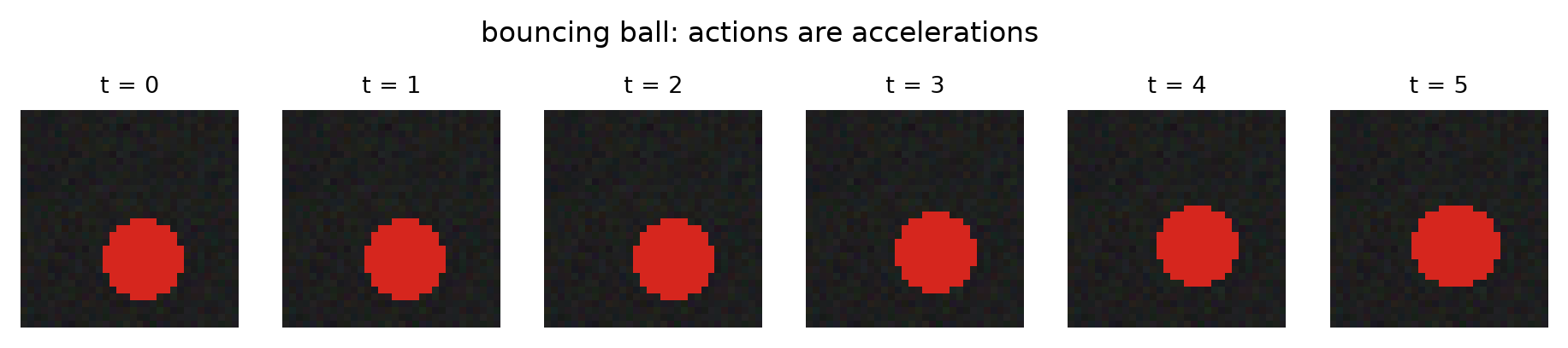
所有模型共用一个 TinyViT:96 维、3 层、4 头、8×8 patch,因此 32×32 的图变成 16 个 patch token,编码器本身约 24.5 万参数;JEPA 加上目标编码器与预测器约 64 万参数。训练在 CPU 上完成,PyTorch 默认线程数为 6。E01 用 6000 张训练图、1500 张测试图、15 个 epoch;参数扫描类实验用 3000 张、8 个 epoch,以便在可接受的时间内跑完六组。所有结果写入 experiments/outputs/metrics.json,正文数字由 R 读取该文件生成。
All models share one TinyViT: 96 dimensions, 3 layers, 4 heads, 8×8 patches, so a 32×32 image becomes 16 patch tokens and the encoder alone has about 245k parameters; JEPA with its target encoder and predictor has about 640k. Training runs on CPU with PyTorch’s default of 6 threads. E01 uses 6000 training images, 1500 test images and 15 epochs; the sweep experiments use 3000 images and 8 epochs so that six configurations finish in reasonable time. All results are written to experiments/outputs/metrics.json, and every number in the text is read from that file by R.
19. 一个最小 ViT / A minimal ViT
编码器的全部内容就是”切块、加位置、过 Transformer、取 CLS”。核心代码不到四十行:
The encoder is nothing more than “cut into patches, add positions, run a Transformer, take the CLS token”. The core is under forty lines:
class TinyViT(nn.Module):
    def __init__(self, dim=96, depth=3, heads=4, patch=8, img=32):
        super().__init__()
        self.patch = patch
        self.grid = img // patch
        self.n_tokens = self.grid * self.grid
        self.patch_embed = nn.Conv2d(3, dim, patch, patch)
        self.cls = nn.Parameter(torch.zeros(1, 1, dim))
        self.pos = nn.Parameter(torch.zeros(1, 1 + self.n_tokens, dim))
        layer = nn.TransformerEncoderLayer(
            d_model=dim, nhead=heads, dim_feedforward=2 * dim,
            dropout=0.0, activation="gelu", batch_first=True, norm_first=True,
        )
        self.blocks = nn.TransformerEncoder(layer, depth, enable_nested_tensor=False)
        self.norm = nn.LayerNorm(dim)

    def patch_tokens(self, x):
        p = self.patch_embed(x).flatten(2).transpose(1, 2)
        return p + self.pos[:, 1:]

    @staticmethod
    def gather_visible(tokens, keep):
        n_keep = int(keep.sum(1)[0].item())
        idx = torch.argsort((~keep).int(), dim=1)[:, :n_keep]
        return torch.gather(tokens, 1, idx.unsqueeze(-1).expand(-1, -1, tokens.size(-1)))

    def forward(self, x, keep=None, return_tokens=False):
        p = self.patch_tokens(x)
        if keep is not None:
            p = self.gather_visible(p, keep)
        cls = self.cls.expand(p.size(0), -1, -1) + self.pos[:, :1]
        t = torch.cat([cls, p], dim=1)
        t = self.norm(self.blocks(t))
        return t if return_tokens else t[:, 0]
形状变化值得逐行对一遍。输入 [B, 3, 32, 32] 经过 Conv2d(3, 96, 8, 8) 变成 [B, 96, 4, 4],flatten(2) 得到 [B, 96, 16],转置后是 [B, 16, 96]。加上位置编码、拼上 CLS,序列长度变成 17。三层之后取第 0 个 token,就是整张图的 96 维摘要。
The shape changes are worth following line by line. The input [B, 3, 32, 32] becomes [B, 96, 4, 4] through Conv2d(3, 96, 8, 8); flatten(2) gives [B, 96, 16] and the transpose gives [B, 16, 96]. With positions and a CLS token the sequence length is 17. After three layers, token 0 is the 96-dimensional summary of the whole image.
gather_visible 是 JEPA 与普通 ViT 的第一个分岔。普通 ViT 看全部 token;JEPA 的上下文编码器只看 keep=True 的位置,所以先把不可见的 token 丢掉,序列长度随掩码比例变化。return_tokens=True 时返回全部 token 而不只是 CLS,因为预测器需要每个位置的编码。目标编码器也复用这个类,只是参数不反传。
gather_visible is the first fork between JEPA and an ordinary ViT. A plain ViT sees all tokens; JEPA’s context encoder sees only keep=True positions, so invisible tokens are dropped and the sequence length varies with the mask ratio. With return_tokens=True the model returns all tokens rather than the CLS, because the predictor needs a code for each position. The target encoder reuses the same class, only without gradients.
20. Predictor 与掩码 / Predictor and masking
掩码决定任务难度。这里用一个尽量简单的策略:在 4×4 的网格上取一个连续矩形,覆盖约 ratio 比例的 patch;如果比例接近 1,则退化为随机选择。True 表示被遮住。
The mask sets the difficulty. The strategy here is deliberately simple: choose a contiguous rectangle on the 4×4 grid covering about ratio of the patches; if the ratio is close to 1, fall back to random selection. True means masked.
def block_mask(batch, grid, ratio, device):
    n = grid * grid
    m = max(1, min(n - 1, int(round(ratio * n))))
    mask = torch.zeros(batch, n, dtype=torch.bool, device=device)
    # find the smallest rectangle with at least m cells
    best = min(((h, w) for h in range(1, grid + 1) for w in range(1, grid + 1)
                if h * w >= m), key=lambda hw: hw[0] * hw[1])
    h, w = best
    for b in range(batch):
        top = torch.randint(0, grid - h + 1, (1,), device=device).item()
        left = torch.randint(0, grid - w + 1, (1,), device=device).item()
        cells = [(top + i) * grid + (left + j)
                 for i in range(h) for j in range(w)][:m]
        mask[b, torch.tensor(cells, device=device)] = True
    return mask
预测器要做的事情是:把可见 token 放回它们原来的位置,在被遮的位置填一个可学习的 mask_token,加上位置编码,过几层 Transformer,最后只输出被遮位置的预测。注意 in_proj/out_proj:预测器的宽度可以和编码器不同,这是故意的瓶颈设计。
What the predictor does: put visible tokens back at their original positions, fill masked positions with a learned mask_token, add positional embeddings, run a few Transformer layers, and output predictions only at masked positions. Note in_proj/out_proj: the predictor width can differ from the encoder width, which is a deliberate bottleneck.
class Predictor(nn.Module):
    def __init__(self, dim=96, depth=2, heads=4, n_tokens=16,
                 width=None, in_dim=None):
        super().__init__()
        width = width or dim
        in_dim = in_dim or dim
        self.in_proj = nn.Linear(in_dim, width) if in_dim != width else nn.Identity()
        self.out_proj = nn.Linear(width, in_dim) if in_dim != width else nn.Identity()
        self.mask_token = nn.Parameter(torch.zeros(1, 1, width))
        self.pos = nn.Parameter(torch.zeros(1, 1 + n_tokens, width))
        layer = nn.TransformerEncoderLayer(
            d_model=width, nhead=heads, dim_feedforward=2 * width,
            dropout=0.0, activation="gelu", batch_first=True, norm_first=True,
        )
        self.blocks = nn.TransformerEncoder(layer, depth, enable_nested_tensor=False)
        self.norm = nn.LayerNorm(width)

    def forward(self, context_tokens, keep):
        context_tokens = self.in_proj(context_tokens)
        B = context_tokens.size(0)
        n = keep.size(1)
        patches = self.mask_token.expand(B, n, -1).clone()
        patches[keep] = context_tokens[:, 1:, :].reshape(-1, context_tokens.size(-1))
        cls = context_tokens[:, :1, :]
        t = torch.cat([cls, patches], dim=1) + self.pos
        t = self.norm(self.blocks(t))
        return self.out_proj(t[:, 1:, :])
patches[keep] = ... 这一行是整段代码里最不直观的。patches 是 [B, 16, width],keep 是 [B, 16] 的布尔矩阵;用布尔索引赋值,相当于把每个样本的 \(K\) 个可见 token 依次写回它们原来的槽位。这样位置信息由槽位本身携带,不必再额外传一个索引张量。最后返回 t[:, 1:, :],丢掉 CLS,只保留 16 个 patch 的预测。
patches[keep] = ... is the least obvious line. patches is [B, 16, width] and keep is a boolean [B, 16] matrix; boolean-indexed assignment writes each sample’s \(K\) visible tokens back into their original slots. Position is then carried by the slot itself, with no extra index tensor. The return t[:, 1:, :] drops the CLS and keeps the 16 patch predictions.
21. 训练循环 / The training loop
训练循环只有十几行,但每一行都对应前面一个概念:
The training loop is a dozen lines, but each line corresponds to a concept above:
def train_jepa(images, epochs=8, mask_ratio=0.5, ema=0.99, reg=0.0,
               predictor_depth=2, predictor_width=96, seed=0, batch=128,
               lr=1e-3, weight_decay=0.05, stop_grad=True):
    torch.manual_seed(seed)
    model = JEPA(predictor_depth=predictor_depth, predictor_width=predictor_width)
    if ema <= 0:
        model.target = model.context          # tied weights: the "joint" regime
    params = list(model.context.parameters()) + list(model.predictor.parameters())
    opt = torch.optim.AdamW(params, lr=lr, weight_decay=weight_decay)
    hist = []
    for ep in range(epochs):
        model.train()
        for (x,) in loader(images, batch=batch):
            mask = block_mask(x.size(0), model.context.grid, mask_ratio, x.device)
            loss, pred = model(x, mask, stop_grad=stop_grad)
            if reg > 0:
                loss = loss + reg * variance_loss(pred.reshape(-1, pred.size(-1)))
            opt.zero_grad()
            loss.backward()
            torch.nn.utils.clip_grad_norm_(params, 1.0)
            opt.step()
            if ema > 0:
                update_ema(model.target, model.context, ema)
            hist.append(loss.item())
    model.eval()
    return model, hist
ema <= 0 这一行是第 24 节六种配置的开关:把 model.target 直接指向 model.context,两个编码器共享参数、没有 stop-gradient 的必要(因为梯度会同时更新”目标”),这就是”联合训练”的坍塌风险版本。reg > 0 加上方差项,stop_grad=False 则连 stop-gradient 也去掉。六种配置就是这三个开关的组合。
The ema <= 0 line is the switch behind the six regimes in Section 24: pointing model.target at model.context ties the two encoders, so there is no point in stop-gradient (the gradient updates the “target” too) — this is the collapse-prone “joint training” version. reg > 0 adds the variance term, and stop_grad=False removes stop-gradient as well. The six regimes are combinations of these three switches.
EMA 更新本身只有三行:
The EMA update itself is three lines:
@torch.no_grad()
def update_ema(target, source, momentum):
    for pt, ps in zip(target.parameters(), source.parameters()):
        pt.data.mul_(momentum).add_(ps.data, alpha=1.0 - momentum)
@torch.no_grad() 既省内存,也防止 EMA 更新被误算进梯度图。mul_ 与 add_ 都是原地操作,所以不会给目标编码器分配新张量。注意这只更新参数,不更新 buffer;本文的模型没有 BatchNorm,所以没有这个问题,但如果换成 ResNet,buffer 也要单独复制。
@torch.no_grad() saves memory and keeps the EMA update out of the gradient graph. Both mul_ and add_ are in-place, so no new tensors are allocated for the target encoder. Note that this updates parameters only, not buffers; the models here have no BatchNorm, so it does not matter, but with a ResNet the buffers would need copying too.
22. 评估代码 / Evaluation code
探针函数把”标准化”和”不标准化”两条路都留着,因为它们的差别在本文里是主角之一:
The probe function keeps both the “standardised” and “raw” paths, because their difference is one of the main characters here:
def probe(features_tr, factors_tr, features_te, factors_te):
    scaler = StandardScaler().fit(features_tr)
    a, b = scaler.transform(features_tr), scaler.transform(features_te)
    res = {}
    for key in ("shape", "colour"):
        clf = LogisticRegression(max_iter=1000)
        clf.fit(a, factors_tr[key])
        res[f"{key}_acc"] = float(clf.score(b, factors_te[key]))
    raw = LogisticRegression(max_iter=1000).fit(features_tr, factors_tr["shape"])
    res["shape_acc_raw"] = float(raw.score(features_te, factors_te["shape"]))
    reg = Ridge(alpha=1.0).fit(a, factors_tr["position"])
    pred = reg.predict(b)
    res["position_rmse"] = float(np.sqrt(np.mean((pred - factors_te["position"]) ** 2)))
    return res
坍塌诊断则把第 14 节的定义直接翻成代码:
The collapse diagnostics translate Section 14’s definitions directly into code:
def collapse_metrics(features):
    f = features.astype(np.float64)
    f = f - f.mean(0, keepdims=True)
    s = np.linalg.svd(f, compute_uv=False)
    p = s / (s.sum() + 1e-12)
    eff_rank = float(np.exp(-np.sum(p * np.log(p + 1e-12))))
    f_norm = f / (np.linalg.norm(f, axis=1, keepdims=True) + 1e-9)
    idx = np.random.default_rng(0).choice(len(f), min(300, len(f)), replace=False)
    cos = f_norm[idx] @ f_norm[idx].T
    off = cos[~np.eye(len(idx), dtype=bool)]
    return {"effective_rank": eff_rank,
            "feature_std": float(f.std(0).mean()),
            "mean_cosine": float(off.mean())}
feature_std 用的是中心化后特征的逐维标准差再取平均,所以它有单位;effective_rank 只看归一化后的奇异值比例,所以它没有单位。把这两个数放在一起看,才能区分”谱很宽但幅度很小”和”谱很窄但幅度正常”。第 24 节的两组数字正好是这两种情况。
feature_std averages per-dimension standard deviations of the centred features, so it carries units; effective_rank uses only normalised singular-value proportions, so it does not. Reading the two together separates “wide spectrum, tiny magnitude” from “narrow spectrum, normal magnitude”. The two groups in Section 24 are exactly these cases.
23. E01:同一躯干,四种目标 / E01: one body, four objectives
第一组实验回答最直接的问题:在完全相同的编码器、数据与训练预算下,把目标函数换掉,表征会差多少? 四个模型共用 TinyViT:JEPA(EMA 0.999、方差正则 0.1、掩码 0.25)、MAE(掩码 0.5、重建像素)、SimCLR(随机裁剪、翻转、亮度,NT-Xent 温度 0.2)、监督学习(三分类交叉熵)。6000 张训练图,1500 张测试图,15 个 epoch,每个模型固定一个随机种子(11–14)。
The first experiment asks the most direct question: with exactly the same encoder, data and training budget, how much does the objective change the representation? Four models share the TinyViT: JEPA (EMA 0.999, variance regulariser 0.1, mask 0.25), MAE (mask 0.5, pixel reconstruction), SimCLR (random crop, flip, brightness; NT-Xent at temperature 0.2), and supervised learning (three-way cross-entropy). 6000 training images, 1500 test images, 15 epochs, one fixed seed per model (11–14).
| 模型 / Model | shape acc | colour acc | position RMSE | effective rank | feature std |
|---|---|---|---|---|---|
| JEPA | 0.606 | 1.000 | 0.103 | 8.78 | 0.185 |
| MAE | 0.588 | 0.992 | 0.067 | 18.04 | 0.211 |
| SimCLR | 0.695 | 1.000 | 0.114 | 12.96 | 0.789 |
| Supervised | 0.957 | 0.983 | 0.103 | 18.90 | 0.789 |
English: shape and colour are three-way and five-way linear probes; position RMSE is in units of image side length; chance is 1/3 for shape and 1/5 for colour.
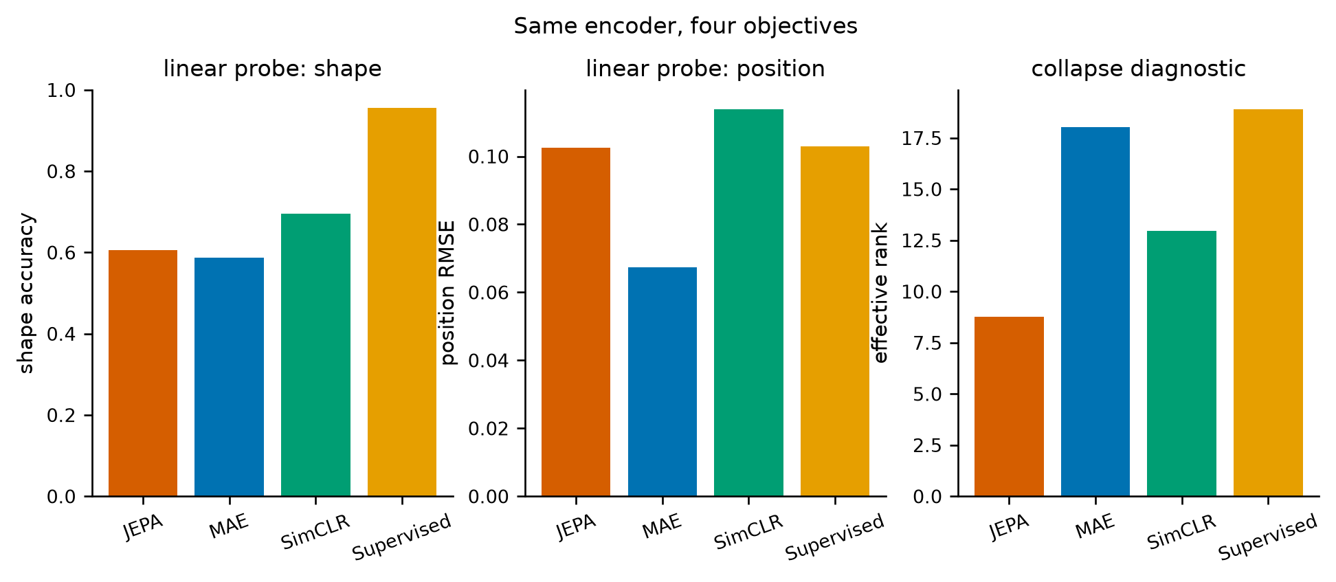
结果很清楚:监督学习以 95.7% 领先,JEPA 只有 60.6%,比 MAE 高 0.018,比 SimCLR 低 0.089。 在自监督三家内部,对比学习最强,JEPA 与像素重建几乎打平。这个结果与”JEPA 应该更好”的预期相反,所以必须认真对待,而不是用”训练不够久”一句话带过。
The result is clear: supervised learning leads at 95.7%; JEPA reaches 60.6%, which is 0.018 above MAE and 0.089 below SimCLR. Among the three self-supervised models, contrastive learning is strongest and JEPA is essentially tied with pixel reconstruction. This contradicts the expectation that JEPA should be better, so it deserves a real explanation rather than “not trained long enough”.
至少有三个原因。第一,规模:I-JEPA 用 ViT-H/14 和数亿张图,本文用 24 万参数的 ViT 和 6000 张图;JEPA 的优势据称来自”丢弃不可预测细节”,而在这个合成数据里几乎没有不可预测细节,像素重建并不吃亏。第二,掩码策略:这里只遮一个矩形块,I-JEPA 用四个大目标块加一个空间分散的上下文块,任务结构完全不同。第三,数据增强:SimCLR 的裁剪与翻转恰好对应”形状不变、位置可变”这个真实因子结构,等于把先验直接写进了任务;JEPA 没有这个先验。
There are at least three reasons. First, scale: I-JEPA uses ViT-H/14 on hundreds of millions of images; here a 245k-parameter ViT sees 6000 images. JEPA’s alleged advantage comes from discarding unpredictable detail, and this synthetic data has almost none, so pixel reconstruction is not penalised. Second, masking: a single rectangle here versus four large target blocks and a spatially distributed context in I-JEPA — a different task. Third, augmentation: SimCLR’s crops and flips match the true factor structure (shape fixed, position varying), effectively writing the prior into the task; JEPA has no such prior.
有效秩一列给出另一条线索。JEPA 的秩是 8.78,四者最低;MAE 与监督学习都在 18 以上。低秩符合”信息瓶颈”的预期:表征被压得很紧。但探针并没有因此变好,说明压缩本身不是目的——压掉的可能是噪声,也可能是类别信息。第 24 节会看到,压缩到极端就是坍塌,两者之间没有一条自动的安全线。
The effective-rank column gives another clue. JEPA’s rank is 8.78, the lowest of the four; MAE and supervised are both above 18. Low rank fits the information-bottleneck story: the representation is tightly compressed. But the probe does not improve, which says compression is not the goal — what gets compressed may be noise or class information. Section 24 shows that the extreme of compression is collapse, with no automatic safe line in between.
24. E02:坍塌的六种命运 / E02: six fates of a joint embedding
第二组只做一件事:把三个开关(是否共享参数、是否用 EMA、是否加方差正则)组合成六种配置,看表征会变成什么样。3000 张图、8 个 epoch、掩码 0.25。这里的 shape_acc_raw 是不标准化的探针,shape_acc 是标准化后的探针;两者一起看,才能识别”有效坍塌”。
The second experiment does one thing: combine three switches (tied weights, EMA, variance regulariser) into six regimes and see what happens to the representation. 3000 images, 8 epochs, mask 0.25. Here shape_acc_raw is the probe without standardisation and shape_acc is the standardised one; reading both is what exposes effective collapse.
| 配置 / Regime | final loss | feature std | effective rank | shape raw | shape std |
|---|---|---|---|---|---|
| joint | 0.00014 | 0.0035 | 40.09 | 0.369 | 0.562 |
| joint + reg 0.1 | 0.0891 | 0.0220 | 19.52 | 0.409 | 0.490 |
| joint + reg 1.0 | 0.0077 | 0.0076 | 17.45 | 0.312 | 0.491 |
| EMA 0.99 | 0.0023 | 0.0476 | 6.29 | 0.380 | 0.547 |
| EMA + reg 0.1 | 0.0927 | 0.0420 | 5.90 | 0.345 | 0.575 |
| EMA 0.999 + reg 0.1 | 0.0919 | 0.1149 | 4.19 | 0.389 | 0.559 |
English: six regimes; raw is the unstandardised probe, std the standardised one; chance is 1/3.
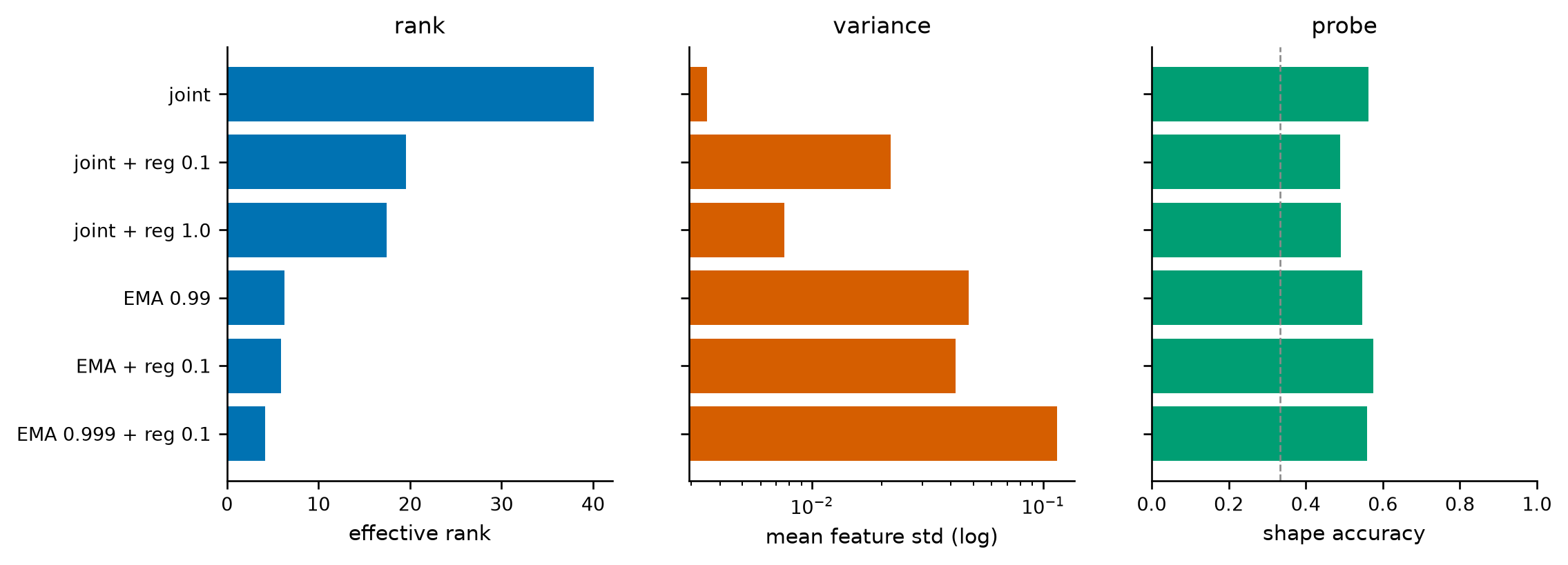
最刺眼的一行是 joint。它的最终损失是 0.00014,几乎是零;有效秩 40.09,是六组里最高的;但特征标准差只有 0.0035,不标准化的探针 0.369,与随机猜(0.333)只差 0.035。标准化之后,同一个模型跳到 0.562——不是因为它突然学到了形状,而是因为 StandardScaler 把 10^{-3} 量级的噪声放大到了单位方差,线性分类器开始在噪声里找边界。
The most striking row is joint. Its final loss is 0.00014, essentially zero; its effective rank is 40.09, the highest of the six; but its feature std is only 0.0035, and the unstandardised probe reaches 0.369, which is 0.035 above chance. After standardisation the same model jumps to 0.562 — not because it suddenly learned shape, but because StandardScaler blows noise of order 10^{-3} up to unit variance and the classifier starts fitting boundaries in that noise.
这是一个方法论上的重要发现,值得单独说:有效秩对尺度不变,所以它无法单独判定坍塌。 一个把整个空间乘以 \(10^{-3}\) 的编码器,秩可以很高,因为秩只看奇异值的相对比例;但所有点都挤在原点附近,线性分类器拿不到任何间隔。要判定坍塌,必须同时看尺度(feature std)与可读性(raw probe)。这也是为什么本文坚持报三个数而不是一个。
This is a methodological finding worth stating separately: effective rank is scale-invariant, so it cannot diagnose collapse on its own. An encoder that multiplies the whole space by \(10^{-3}\) can have high rank, because rank sees only relative singular values; but all points sit near the origin and a linear classifier has no margin. Diagnosing collapse requires scale (feature std) and readability (raw probe) together. That is why three numbers are reported here rather than one.
EMA 的两行给出另一种图景。\(m=0.99\) 把秩压到 6.29,把标准差抬到 0.0476,raw 探针 0.380;加上正则后 raw 反而略降。\(m=0.999\) 的一行标准差最大(0.1149),秩最小(4.19),但 raw 探针只有 0.389。用第 15 节的话说:在这个只有几百步的训练里,\(m=0.999\) 的目标几乎是初始编码器,预测器面对的是一个”几乎不动”的靶子,任务太容易,学不到有用的东西。EMA 不是越慢越好。
The two EMA rows give a different picture. \(m=0.99\) pushes rank down to 6.29 and std up to 0.0476, with a raw probe of 0.380; adding the regulariser slightly lowers the raw probe. The \(m=0.999\) row has the largest std (0.1149), the smallest rank (4.19), yet a raw probe of only 0.389. In the language of Section 15: over a few hundred steps, an \(m=0.999\) target is almost the initial encoder, the predictor faces a nearly frozen target, the task is too easy, and nothing useful is learned. Slower EMA is not automatically better.
25. E03:掩码比例 / E03: mask ratio
第三组扫掩码比例。JEPA 与 MAE 各跑 0.25、0.5、0.75 三档,其他设置相同(3000 张图、8 个 epoch)。0.25 意味着只遮 4 个 patch,0.5 遮 8 个,0.75 遮 12 个;上下文分别剩 12、8、4 个。
The third experiment sweeps the mask ratio. JEPA and MAE each run 0.25, 0.5 and 0.75 with otherwise identical settings (3000 images, 8 epochs). A ratio of 0.25 masks 4 patches, 0.5 masks 8 and 0.75 masks 12; the context keeps 12, 8 and 4 respectively.
| 模型 / Model | ratio | shape std | shape raw | effective rank | position RMSE |
|---|---|---|---|---|---|
| JEPA | 0.25 | 0.589 | 0.509 | 6.54 | 0.074 |
| JEPA | 0.50 | 0.580 | 0.350 | 13.99 | 0.097 |
| JEPA | 0.75 | 0.547 | 0.411 | 5.34 | 0.102 |
| MAE | 0.25 | 0.536 | 0.370 | 5.25 | 0.080 |
| MAE | 0.50 | 0.556 | 0.388 | 5.46 | 0.079 |
| MAE | 0.75 | 0.552 | 0.461 | 3.06 | 0.073 |
English: both models across three mask ratios; raw is the unstandardised probe; chance is 1/3.
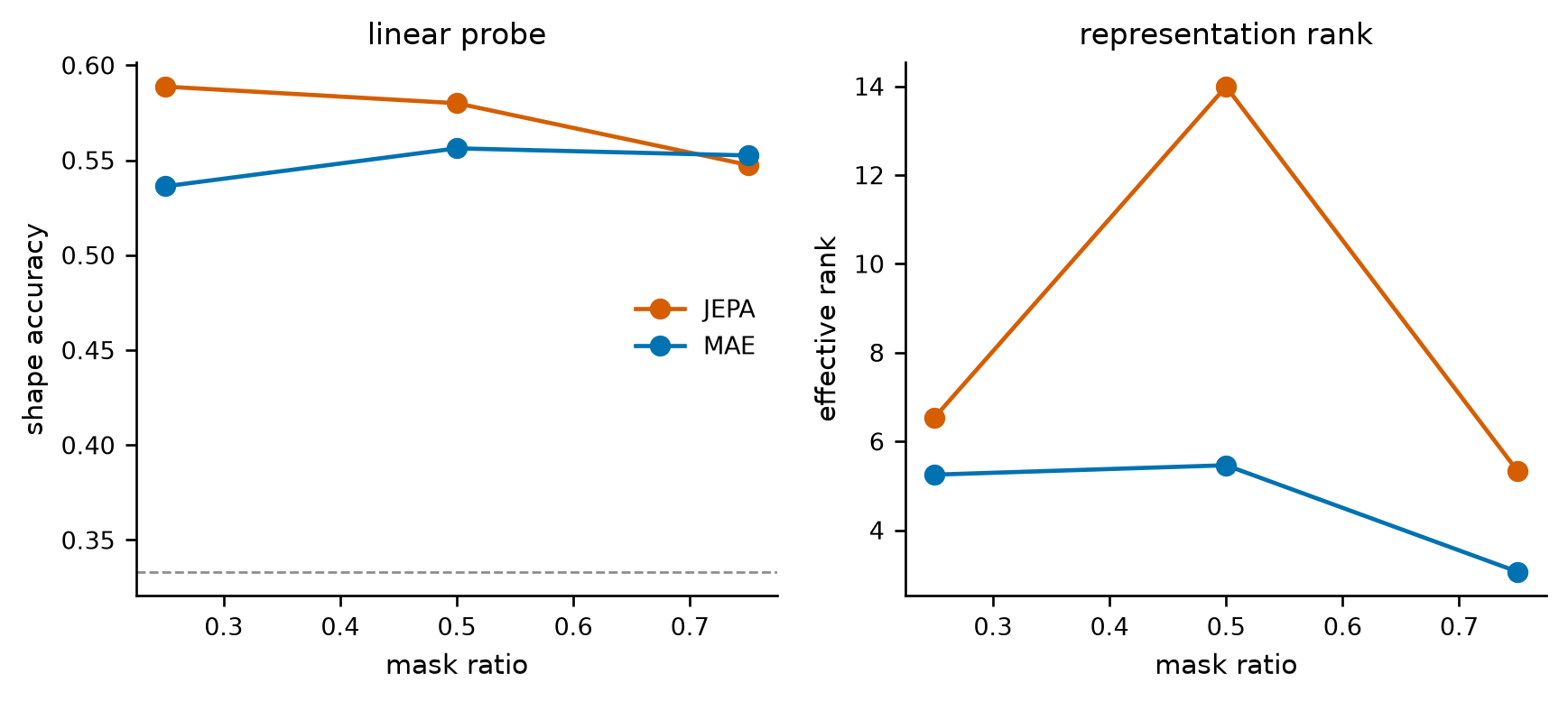
先看 JEPA。标准化探针从 0.589 降到 0.580 再到 0.547,单调下降;raw 探针却是 0.509、0.350、0.411,中间低两头高。有效秩在 0.5 时跳到 13.99,是六格里的最高值,但同一格的 raw 探针最低。MAE 则几乎平坦,三档都在 0.536 到 0.556 之间。
Start with JEPA. The standardised probe falls monotonically from 0.589 to 0.580 to 0.547; the raw probe is 0.509, 0.350, 0.411 — lowest in the middle. Rank jumps to 13.99 at 0.5, the highest of the six cells, while the raw probe in that same cell is the lowest. MAE is almost flat, between 0.536 and 0.556.
怎么解释这种不同步?一种可能性是任务难度与可学信号之间的权衡。0.25 时上下文有 12 个 patch,信息足够,预测器容易学,表征的尺度也正常;0.5 时上下文减半,预测误差变大,编码器被迫展开更多方向(秩升高),但尺度变小(raw 探针下降);0.75 时只剩 4 个 patch,任务接近”从一个角猜全图”,编码器学到的是位置先验而不是形状,raw 探针反而回升一点。这不是一条定理,而是一个在 3000 张图、8 个 epoch 下观察到的现象。换种子、换数据规模,排序可能变。
How to explain the mismatch? One possibility is a trade-off between task difficulty and learnable signal. At 0.25 the context has 12 patches, information is sufficient, the predictor learns easily and the scale stays normal; at 0.5 the context halves, prediction error grows, the encoder is forced to spread into more directions (rank up) but the scale shrinks (raw probe down); at 0.75 only 4 patches remain, the task is close to “guess the whole image from one corner”, the encoder learns a position prior rather than shape, and the raw probe recovers slightly. This is not a theorem but an observation at 3000 images and 8 epochs; another seed or scale could reorder the rows.
和 I-JEPA 的差别也要说清。I-JEPA 用的不是单矩形掩码,而是四个大目标块,总遮蔽比例常到 0.85,同时要求上下文块在空间上分散。它报告的两个关键设计条件是”目标块足够大”和”上下文足够有信息”,而这两条都不是”比例”一个数能概括的。把比例从 0.25 扫到 0.75,只扫到了这条设计空间的一维切片;切片上的非单调,不足以否定原论文的结论。
The difference from I-JEPA should also be stated. I-JEPA does not use one rectangular mask but four large target blocks, often covering around 0.85 of the image, while requiring a spatially distributed context. Its two stated design conditions are “target blocks large enough” and “context informative enough”, and neither is captured by a single ratio. Sweeping the ratio from 0.25 to 0.75 samples a one-dimensional slice of that design space; non-monotonicity on the slice does not refute the original paper.
26. E04:预测器的容量 / E04: predictor capacity
第四组只改预测器:深度取 1、2、3,宽度取 64、128、256,组合成六种配置,其他不变。预测器是 JEPA 里最容易被忽视的零件——它不接触像素,只在表征空间里工作,但它的容量决定了”上下文信息能被推到多远”。
The fourth experiment changes only the predictor: depth 1, 2, 3 and width 64, 128, 256, six combinations, everything else fixed. The predictor is the most easily overlooked part of JEPA — it never touches pixels and works only in representation space — but its capacity decides how far context information can be pushed.
| 深度 / depth | 宽度 / width | shape std | shape raw | position RMSE |
|---|---|---|---|---|
| 1 | 64 | 0.562 | 0.439 | 0.084 |
| 2 | 64 | 0.593 | 0.427 | 0.091 |
| 3 | 64 | 0.549 | 0.431 | 0.087 |
| 2 | 128 | 0.584 | 0.436 | 0.090 |
| 3 | 128 | 0.601 | 0.372 | 0.093 |
| 2 | 256 | 0.583 | 0.534 | 0.085 |
English: six predictor configurations; the encoder and data are identical across rows.
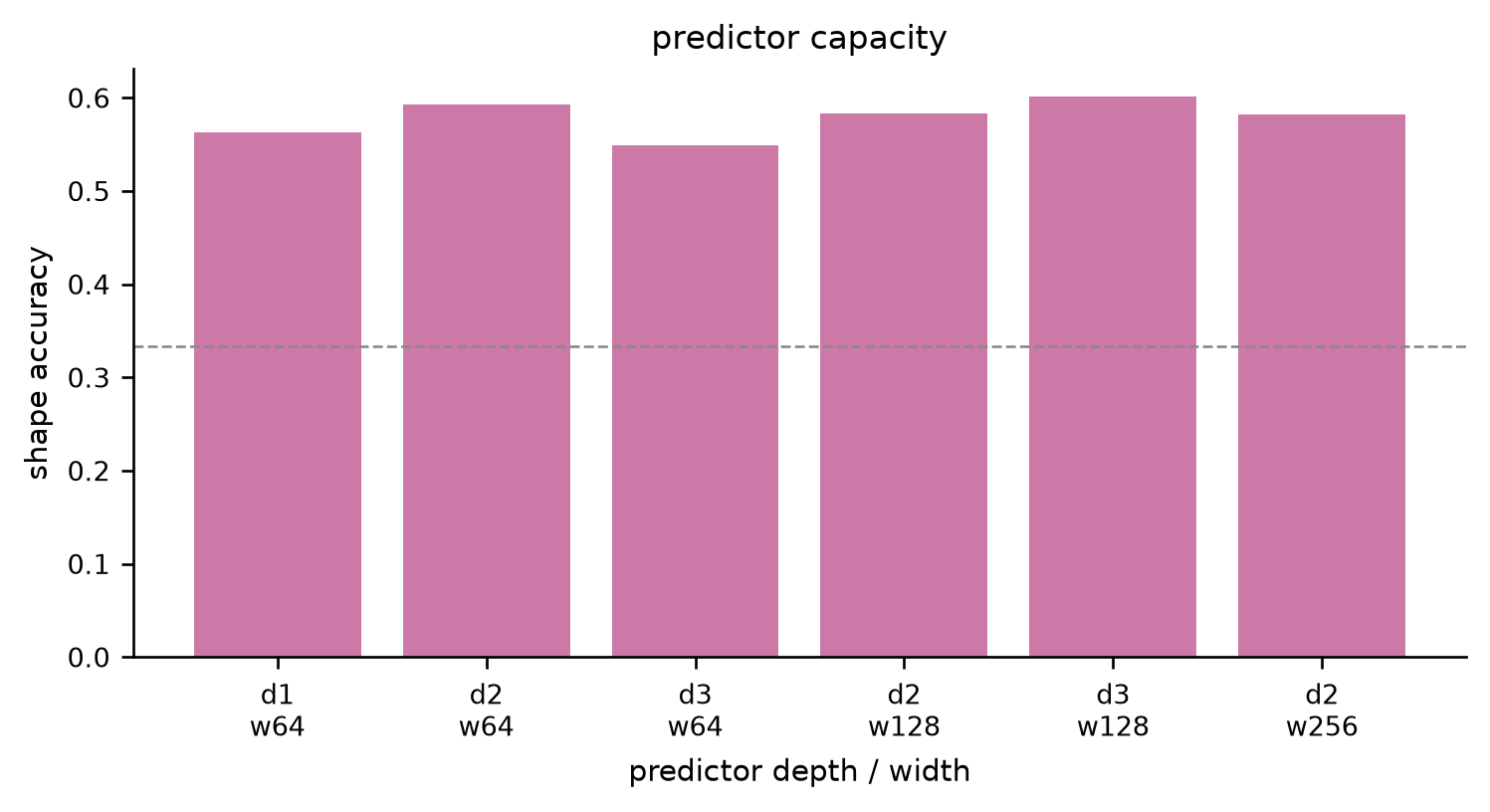
六组结果挤在 0.549 到 0.601 之间,起伏约 0.052。最高的一个是深度 3、宽度 128(0.601),最低的是深度 3、宽度 64(0.549)——深度相同,宽度翻倍反而更好,但深度 2、宽度 64 又有 0.593,比深度 3、宽度 64 高。没有一条”越深越宽越好”的曲线,也没有”越浅越好”的反向曲线。
The six results sit between 0.549 and 0.601, a spread of about 0.052. The best is depth 3, width 128 (0.601); the worst is depth 3, width 64 (0.549) — same depth, doubled width helps, but depth 2, width 64 reaches 0.593, above depth 3, width 64. There is neither a “deeper and wider is better” curve nor the reverse.
最合理的读法是:在这个尺度上,预测器容量不是瓶颈。 数据只有 3000 张、编码器只有 3 层、任务只有 16 个 patch,“从 12 个可见 patch 推到 4 个被遮 patch”所需的关系并不复杂;把它做得更深更宽,多出来的参数主要在拟合噪声。这也符合 JEPA 的设计哲学:预测器应该弱到不能独自解决问题,否则它会绕开编码器,把任务变成一个普通的回归问题。
The most reasonable reading: at this scale, predictor capacity is not the bottleneck. With 3000 images, a 3-layer encoder and 16 patches, the relation needed to go from 12 visible patches to 4 masked ones is not complex; extra depth and width mostly fit noise. This also fits the design philosophy: the predictor should be too weak to solve the task alone, otherwise it bypasses the encoder and turns the problem into ordinary regression.
必须承认这组实验的证据强度有限。六个配置、一个种子、每个数字只来自 800 张测试图,准确率的标准误约 0.018,而极差只有 0.052。换句话说,这些差异很可能大部分是噪声。它足以说明”没有强烈单调趋势”,不足以说明”容量完全无关”。
The evidence here is admittedly weak. Six configurations, one seed, 800 test images per number put the standard error of an accuracy near 0.018, while the full range is only 0.052. In other words, most of these differences are probably noise. That is enough to say “no strong monotone trend” and not enough to say “capacity is irrelevant”.
27. E05:视频世界模型与 rollout / E05: a video world model and rollout
第五组把 JEPA 从静态图像移到视频。训练两个世界模型:JEPA 版用目标编码器编码下一帧,预测器接收当前帧 token 与动作,输出下一帧的 16 个 patch 编码;像素版结构相同,但最后用一个线性头把 token 解码成 3×8×8 的像素块,损失是像素 MSE。两者都用 1600 条 8 帧视频、5 个 epoch。
The fifth experiment moves JEPA from still images to video. Two world models are trained: the JEPA version encodes the next frame with the target encoder, and a predictor takes current-frame tokens plus an action and outputs 16 patch codes for the next frame; the pixel version has the same structure but a linear head decodes tokens into 3×8×8 pixel blocks with an MSE loss. Both use 1600 eight-frame clips for 5 epochs.
rollout 的做法是自回归:从第一帧的编码开始,每一步用预测出的 token 替换 patch token 部分、保留 CLS,再把新的 token 序列喂回预测器。误差在第 \(h\) 步定义为预测 token 与目标编码器对真实第 \(h\) 帧编码之间的均方误差;图中报的是前 \(h\) 步的平均。
Rollout is autoregressive: start from the first frame’s encoding, and at each step replace the patch-token part with the prediction while keeping the CLS, then feed the new sequence back. The error at step \(h\) is the mean squared difference between the predicted tokens and the target encoder’s code for the true frame \(h\); the figure reports the average over the first \(h\) steps.
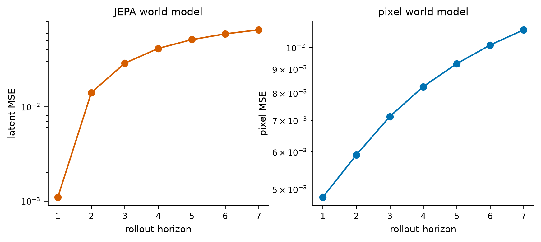
JEPA 版的误差从第 1 步的 0.0011 升到第 7 步的 0.0652,约 59.6 倍;像素版从 0.0048 升到 0.0109,约 2.27 倍。两条曲线都没有爆炸,但都在稳步上升,说明单步训练的模型在多步 rollout 下会积累误差。JEPA 版的相对增长更快,一部分原因是它的初始误差就小得多(分母小),另一部分是目标编码器会随着输入变化而移动,预测器追的是一个移动靶。
The JEPA version rises from 0.0011 at step 1 to 0.0652 at step 7, about 59.6×; the pixel version from 0.0048 to 0.0109, about 2.27×. Neither explodes, but both climb steadily, showing that a model trained on one step accumulates error over many. The JEPA curve grows faster in relative terms partly because it starts much lower (a smaller denominator), and partly because the target encoder moves with the input, so the predictor chases a moving target.
这里有一个必须说清的陷阱:潜空间的 MSE 不是物理误差。 两个状态在表征空间里距离很小,可能对应完全不同的球位置;反过来,同一个位置在不同光照下也可能距离很大。第 28 节的规划失败,正是这个陷阱的直接后果。要判断世界模型是否真的学到了物理,需要把潜状态解码回位置与速度,或者直接用真实状态算误差;本文没有做这件事,所以第 27 节只能支持”误差没有爆炸”,不能支持”模型理解了弹球”。
A trap must be stated: latent MSE is not physical error. Two states can be close in representation space while corresponding to very different ball positions, and the same position under different lighting can be far apart. The planning failure in Section 28 is a direct consequence. To know whether the world model learned the physics, one must decode latent states back to position and velocity, or compute error on the true state; that was not done here, so Section 27 supports “the error does not explode”, not “the model understands the ball”.
28. E06:潜空间规划 / E06: planning in latent space
第六组用第 27 节的两个世界模型做规划。每一回合:球从 \([0.25,0.75]^2\) 内随机位置、零速度出发,目标位置在 \([0.2,0.8]^2\) 内随机抽取并渲染成一张目标帧;控制器连续执行 12 步,每一步用 CEM 在长度为 5 的动作序列上搜索(种群 24、迭代 3 轮、精英 6 条),只执行第一个动作,下一步重新规划;12 步后若球心与目标的距离小于 0.08,记为成功。跑 10 个回合,比较三种策略:潜空间规划、像素空间规划、随机动作。
The sixth experiment plans with the two world models from Section 27. Each episode: the ball starts at a random position in \([0.25,0.75]^2\) with zero velocity, and a goal position is drawn uniformly from \([0.2,0.8]^2\) and rendered as a goal frame. The controller runs 12 steps; at each step CEM searches over action sequences of length 5 (population 24, 3 iterations, 6 elites), only the first action is executed, and planning repeats. After 12 steps, a final distance below 0.08 counts as success. Over 10 episodes, three strategies are compared: latent planning, pixel planning and random actions.
| 策略 / Strategy | 成功率 / success | 最终距离 / final distance |
|---|---|---|
| 潜空间规划 / latent | 0.0 | 0.383 |
| 像素空间规划 / pixel | 0.0 | 0.337 |
| 随机动作 / random | 0.1 | 0.368 |
English: success is the fraction of episodes ending within the threshold; distance is the final distance to the goal, lower is better.
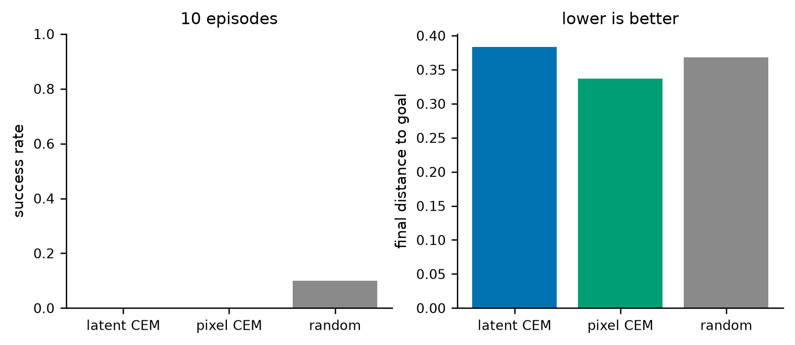
结果必须原样报告:潜空间规划成功率 0.0,像素空间 0.0,随机动作 0.1;最终距离分别是 0.383、0.337、0.368。 潜空间规划不仅没赢,还比随机差 0.015。像素规划距离最好,但也没有一次达到阈值。
The result must be reported as it is: latent planning succeeds 0.0 of the time, pixel planning 0.0, random actions 0.1; final distances are 0.383, 0.337 and 0.368. Latent planning does not merely fail to win; it ends 0.015 further than random. Pixel planning has the best distance but never crosses the threshold either.
原因至少有五条,按我判断的重要性排序。第一,代价函数错位:潜空间欧氏距离不度量物理距离,CEM 会找到”表征上接近但状态上不对”的动作序列,这正是第 17 节警告的风险。第二,单步模型:训练只教了”给定当前帧与动作,下一帧是什么”,没有教多步复合;CEM 却要用它滚 5 步。第三,目标表征可能丢位置:如果目标编码器主要保留形状与颜色,位置信息在目标里就很弱,规划等于在追一个不含位置的靶。第四,搜索预算太小:24×3 的 CEM 在二维、5 步的连续空间里只探索了很少的样本。第五,成功阈值:0.08 的距离阈值相对于 12 步内能走到的范围可能过严,像素规划距离最好却仍是 0 成功率,说明阈值本身也需要检查。
There are at least five reasons, ordered by how much I think they matter. First, the cost is mismatched: Euclidean distance in latent space does not measure physical distance, so CEM finds sequences that are close in representation but wrong in state — exactly the risk flagged in Section 17. Second, the model is one-step: training only says “given this frame and action, here is the next frame”, never multi-step composition, yet CEM rolls it five steps. Third, the goal code may lose position: if the target encoder mostly keeps shape and colour, position is weak in the target and planning chases a target without position. Fourth, the search budget is tiny: a 24×3 CEM explores very few samples in a two-dimensional, five-step continuous space. Fifth, the success threshold: a distance of 0.08 may be too strict for what 12 steps can reach, since pixel planning has the best distance and still zero success.
这个负面结果的价值在于它精确地指出了”潜空间规划”不是免费的。LeCun 的蓝图里,规划之所以可行,是因为世界模型的潜空间保留了与任务相关的状态变量,并且代价函数定义在这个空间里;本文的玩具模型两条都不满足。它不构成对 JEPA 的反驳,但它构成对一个常见口号的提醒:“在潜空间里规划更快”只有在潜空间真的包含规划所需的信息时才成立。
The value of this negative result is that it pins down why “planning in latent space” is not free. In LeCun’s blueprint, planning works because the world model’s latent space retains the state variables relevant to the task and the cost is defined in that space; the toy model here satisfies neither. This is not a refutation of JEPA, but it is a warning about a common slogan: “planning in latent space is faster” holds only when the latent space actually contains what planning needs.
29. E07:分布外 / E07: out of distribution
最后一组测泛化。训练集不变,测试集换成分布外版本:背景亮度从 0.05–0.25 抬到 0.35–0.65,颜色换成另一套调色板,半径整体放大或缩小,噪声标准差从 0.015 升到 0.06。探针仍然只在分布内数据上训练,然后直接拿到分布外数据上测。
The last experiment tests generalisation. Training data are unchanged; the test set is an out-of-distribution version: background brightness raised from 0.05–0.25 to 0.35–0.65, a different colour palette, radius scaled up or down, and noise standard deviation raised from 0.015 to 0.06. Probes are still trained on in-distribution data and evaluated directly out of distribution.
| 模型 / Model | 形状 ID / shape ID | 形状 OOD / shape OOD | 颜色 ID / colour ID | 颜色 OOD / colour OOD | 位置 OOD / position OOD |
|---|---|---|---|---|---|
| JEPA | 0.600 | 0.361 | 0.999 | 0.119 | 0.173 |
| MAE | 0.580 | 0.314 | 0.990 | 0.091 | 0.284 |
| SimCLR | 0.669 | 0.384 | 1.000 | 0.228 | 0.255 |
| Supervised | 0.954 | 0.380 | 0.975 | 0.282 | 0.175 |
English: ID is in-distribution, OOD is the shifted test set; chance is 1/3 for shape and 1/5 for colour.
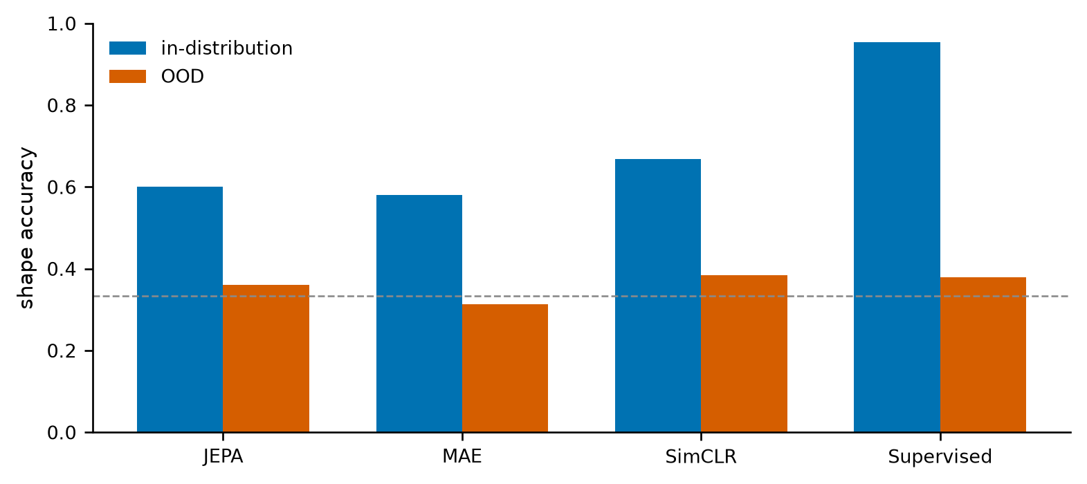
形状上,四个模型在分布外全部跌到随机水平附近:JEPA 0.600 → 0.361,MAE 0.580 → 0.314,SimCLR 0.669 → 0.384,监督学习 0.954 → 0.380。颜色更糟:分布内几乎都是 1.0,分布外分别是 0.119、0.091、0.228、0.282,前两个低于 0.2 的随机水平。
On shape, all four fall to near chance out of distribution: JEPA 0.600 → 0.361, MAE 0.580 → 0.314, SimCLR 0.669 → 0.384, supervised 0.954 → 0.380. Colour is worse: near 1.0 in distribution, and 0.119, 0.091, 0.228, 0.282 out of distribution — the first two below the 0.2 chance level.
低于随机不是”忘了颜色”,而是系统性地把颜色映射错。线性分类器的决策边界是在旧调色板上切的;新调色板的五个颜色落在旧边界的另一侧,分类器仍然自信地给出旧标签,于是准确率可以低于均匀猜测。这提醒我们:OOD 准确率低于随机,说明错误是结构性的,不是噪声。 位置也变差,但没有颜色那么极端:JEPA 从 0.106 升到 0.173,监督学习从 0.105 升到 0.175。
Below chance is not “forgetting colour” but systematically mis-mapping it. The linear boundary was cut on the old palette; the five new colours fall on the other side of the old boundary, the classifier still answers confidently with old labels, and accuracy can end up below uniform guessing. This is a reminder: OOD accuracy below chance means the error is structural, not noise. Position degrades too, though less extremely: JEPA goes from 0.106 to 0.173, supervised from 0.105 to 0.175.
最重要的一点是:JEPA 没有表现出更强的分布外不变性。 它和 MAE、SimCLR 一样跌,甚至颜色跌得比 SimCLR 更狠。原因不神秘:本文的 JEPA 没有任何颜色增强,目标编码器也没有被要求忽略颜色,所以它没有任何理由学出颜色不变性。不变性不会从”预测表征”这个动作里自动长出来;它是数据、增强与目标共同塑造的。这条结论与第 23 节一致:目标函数决定表征里有什么,但决定不了表征里没有什么。
The most important point: JEPA shows no stronger out-of-distribution invariance. It falls like MAE and SimCLR, and on colour falls harder than SimCLR. The reason is not mysterious: this JEPA has no colour augmentation and no pressure on the target encoder to ignore colour, so it has no reason to learn colour invariance. Invariance does not emerge automatically from “predict a representation”; it is shaped by data, augmentations and objective together. This matches Section 23: the objective decides what is in the representation, but not what is absent from it.
30. 这些实验不能证明什么 / What these experiments do not show
把边界说清楚,比把结论说大更重要。第一,规模。本文的编码器约 24.5 万参数,数据 3000–6000 张,训练 8–15 个 epoch;I-JEPA 用 ViT-H/14 与数亿张图,V-JEPA 2 用超过一百万小时视频。JEPA 的许多性质被报告为”随规模出现”,玩具实验看不到它们,是意料之中的。
Stating the limits matters more than inflating the conclusions. First, scale. The encoder here has about 245k parameters, the data 3000–6000 images, and training 8–15 epochs; I-JEPA uses ViT-H/14 on hundreds of millions of images and V-JEPA 2 uses over a million hours of video. Many JEPA properties are reported to emerge with scale, so a toy experiment not seeing them is expected.
第二,单一随机种子。所有实验都只跑一个种子(E01 的四个模型各用一个不同的种子);E04 的极差已经在标准误附近,其他组的排序也可能翻转。第三,合成数据。图形与弹球没有真实图像的纹理、光照、遮挡,也没有真实视频的长程语义;在这里成立的结论,不能直接搬到 ImageNet 或机器人。第四,探针不是下游。线性探针只测”信息是否线性可读”,不测检测、分割、控制;一个探针低的表征可能在下游微调后很好,反之亦然。
Second, a single seed. Every experiment runs one seed (the four models in E01 use four different seeds); the spread in E04 is already near the standard error and other rankings could flip. Third, synthetic data. Shapes and bouncing balls lack real texture, lighting and occlusion, and lack the long-range semantics of real video; conclusions here do not transfer directly to ImageNet or robots. Fourth, a probe is not a downstream task. It measures linear readability, not detection, segmentation or control; a low-probe representation may fine-tune well, and vice versa.
那么这些实验能证明什么?它们能证明机制的存在:联合训练确实会把表征推向低方差,标准化确实会掩盖这一点,掩码比例确实会改变秩与可读性,单步世界模型确实会在多步 rollout 中积累误差,潜空间距离确实不等于物理距离。这些是设计 JEPA 时必须面对的事实,不依赖于模型多大。它们不能证明JEPA 在规模上是否优于其他目标——那是另一类实验,需要另一套预算。
So what do they show? They show that the mechanisms exist: joint training really does push representations toward low variance, standardisation really does hide it, mask ratio really does change rank and readability, a one-step world model really does accumulate error over rollout, and latent distance really is not physical distance. These are facts any JEPA design must face, independent of model size. They do not show whether JEPA beats other objectives at scale — that is a different experiment with a different budget.
31. I-JEPA:图像上的第一次落地 / I-JEPA: the first landing on images
I-JEPA(2023)把立场文章里的方块第一次变成可训练的模型。做法是:从一张图里取一个上下文块,再取四个目标块,用上下文编码器编码前者,用目标编码器编码后者,预测器根据上下文和”目标块的位置”输出四个块的预测。关键设计不是损失,而是掩码:目标块要足够大,才携带语义;上下文块要空间分散,才提供足够信息。论文报告,用 ViT-Huge/14 在 16 张 A100 上不到 72 小时就能完成 ImageNet 预训练。
I-JEPA (2023) turned the blueprint’s box into a trainable model for the first time. It takes one context block and four target blocks from an image, encodes the former with the context encoder and the latter with the target encoder, and a predictor outputs the four target codes conditioned on the context and the positions of the target blocks. The key design is not the loss but the masking: target blocks must be large enough to carry semantics, and the context must be spatially distributed enough to be informative. The paper reports ImageNet pre-training with ViT-Huge/14 on 16 A100s in under 72 hours.
它的意义有三层。第一,证明非生成式自监督可以在规模上工作:不需要重建像素,不需要手工增强,也能得到可迁移的图像表征。第二,把”预测什么”变成主要设计变量:此前的自监督方法主要在比较损失(对比、重建、蒸馏),I-JEPA 把注意力引到”目标块怎么选”。第三,给出了一个可复用的模板:两个编码器、一个预测器、一个掩码策略,之后的 V-JEPA 与 V-JEPA 2 都沿用这个骨架。
Its significance is threefold. First, it shows that non-generative SSL works at scale: no pixel reconstruction and no hand-crafted augmentations are needed to obtain transferable image representations. Second, it makes “what to predict” the main design variable: earlier SSL mostly compared losses (contrastive, reconstruction, distillation), while I-JEPA points at how target blocks are chosen. Third, it provides a reusable template: two encoders, one predictor, one masking strategy — the skeleton that V-JEPA and V-JEPA 2 keep.
需要克制的一点是:I-JEPA 的强项被报告在下游任务上(线性分类、物体计数、深度预测),而不是某个单一数字。本文没有复现它的规模,所以第 23 节的负面结果与它并不矛盾:一个在 6000 张合成图上、用单矩形掩码、训练 15 个 epoch 的 JEPA,本来就不该被期待复现 ViT-H/14 的行为。
One restraint is needed: I-JEPA’s strengths are reported on downstream tasks (linear classification, object counting, depth prediction) rather than on a single headline number. This article does not reproduce its scale, so the negative result in Section 23 does not contradict it: a JEPA trained on 6000 synthetic images with a single rectangular mask for 15 epochs should not be expected to reproduce ViT-H/14 behaviour.
32. V-JEPA 家族:视频、规模与机器人 / The V-JEPA family: video, scale and robots
V-JEPA(2024)把同一套目标搬到视频。输入不再是单张图,而是时空立方体;掩码变成时空管,预测器要预测被遮住的时空区域在目标编码器里的表征。训练完的编码器冻结后用于评估,论文报告 ViT-H/16 在 Kinetics-400 上 81.9、Something-Something v2 上 72.2、ImageNet-1K 上 77.9。这些数字的意义不是”最高”,而是”一个不做像素重建、不做对比负样本的模型,可以在视频动作识别上接近当时的强基线”。
V-JEPA (2024) moves the same objective to video. The input is a spatio-temporal volume rather than a single image; masks become tubes, and the predictor must predict the target encoder’s representation of the masked region. The trained encoder is evaluated frozen; the paper reports ViT-H/16 at 81.9 on Kinetics-400, 72.2 on Something-Something v2 and 77.9 on ImageNet-1K. The point is not “state of the art” but that a model with no pixel reconstruction and no contrastive negatives can come close to strong video baselines.
V-JEPA 2(2025)把规模和数据推上一个量级:超过一百万小时的互联网视频,加上少量机器人轨迹。它报告 Something-Something v2 上 77.3、Epic-Kitchens-100 动作预测 39.7 recall-at-5;接上大语言模型后,在 80 亿参数规模上报告 PerceptionTest 84.0、TempCompass 76.9。更重要的是 V-JEPA 2-AC:用不到 62 小时的 Droid 无标注机器人视频后训练一个动作条件世界模型,在两个实验室的 Franka 机械臂上零样本执行抓放,不需要目标环境的任何数据、任务训练或奖励。
V-JEPA 2 (2025) pushes scale and data up an order of magnitude: over a million hours of internet video plus a small amount of robot trajectories. It reports 77.3 on Something-Something v2 and 39.7 recall-at-5 on Epic-Kitchens-100 action anticipation; aligned with a large language model at the 8-billion-parameter scale, it reports 84.0 on PerceptionTest and 76.9 on TempCompass. More importantly, V-JEPA 2-AC post-trains an action-conditioned world model on under 62 hours of unlabelled Droid robot video and performs pick-and-place zero-shot on Franka arms in two laboratories, with no data from those environments, no task training and no reward.
V-JEPA 2.1(2026)是这条线的继续。它加入稠密预测损失(不只预测被遮块,而是让每个位置都参与)、深层自监督(不只监督最后一层)与多模态 tokenizer,把同一骨架扩展到更多输入类型。报告的数字包括 Ego4D 7.71 mAP、Epic-Kitchens-100 40.8 recall-at-5、Something-Something v2 77.7、NYUv2 深度 0.307 RMSE、TartanDrive 5.687 ATE,以及抓取任务上约 20 个点的提升。这些数字分散在感知、深度、导航与操作四类任务上,说明它想证明的不是单点最强,而是一个世界模型可以同时支撑多种下游。
V-JEPA 2.1 (2026) continues the line. It adds a dense predictive loss (every position participates, not only masked blocks), deep self-supervision (more than the last layer is supervised) and multi-modal tokenizers, extending the skeleton to more input types. Reported numbers include 7.71 mAP on Ego4D, 40.8 recall-at-5 on Epic-Kitchens-100, 77.7 on Something-Something v2, 0.307 RMSE on NYUv2 depth, 5.687 ATE on TartanDrive, and roughly a 20-point gain on a grasping task. Spread across perception, depth, navigation and manipulation, they argue not for a single best number but for one world model supporting many downstream tasks.
这条线最重要的转变是评价对象变了:I-JEPA 问”表征好不好”,V-JEPA 2 问”能不能用来规划”,V-JEPA 2.1 问”一个模型能覆盖多少种任务”。评价从线性探针移到了机器人成功率与导航误差,这是好事,因为探针会饱和;但也带来新问题:机器人实验难以复现,数据与硬件门槛高,负面结果不容易发表。第 28 节的玩具规划失败,在真实系统里可能被工程细节掩盖,也可能被更严格的评测放大。
The most important shift is what is being evaluated: I-JEPA asks “is the representation good”, V-JEPA 2 asks “can it be used to plan”, V-JEPA 2.1 asks “how many tasks can one model cover”. Evaluation moves from linear probes to robot success rates and navigation error, which is good because probes saturate; but it brings new problems: robot experiments are hard to reproduce, the data and hardware bar is high, and negative results are hard to publish. The toy planning failure in Section 28 could be hidden by engineering details in a real system, or amplified by stricter evaluation.
33. LeJEPA 与 LeWorldModel:去掉启发式 / LeJEPA and LeWorldModel: removing the heuristics
LeJEPA(2025)针对的是 JEPA 最尴尬的部分:stop-gradient、EMA、teacher-student、冷启动、掩码调度,这些技巧在论文里被反复调,却缺少一个统一解释。LeJEPA 提出 SIGReg:用随机投影把嵌入投到若干一维方向,要求每个投影的分布接近标准正态。各向同性高斯既不会坍塌(方差不会掉到零),也不会把信息挤在少数方向(协方差接近单位阵)。论文主张这套目标只需要一个权衡超参数,并在 60 多种架构上验证线性探针的表现。
LeJEPA (2025) targets JEPA’s most awkward part: stop-gradient, EMA, teacher-student, warm-up and mask schedules are tuned repeatedly in papers without a unified explanation. LeJEPA proposes SIGReg: random projections map the embedding to several one-dimensional directions, and each projected distribution is pushed toward a standard normal. An isotropic Gaussian neither collapses (variance does not go to zero) nor squeezes information into a few directions (covariance near identity). The paper argues that this objective needs a single trade-off hyperparameter and validates linear-probe performance across more than 60 architectures.
LeWorldModel(2026)走的是另一条路:把世界模型做小。它报告约 1500 万参数、单张 GPU 数小时训练、只有两个损失项,并在规划任务上报告最高 48 倍的加速。这个工作的意义不在于刷新某个 benchmark,而在于把”JEPA 世界模型”从需要工业级预算的东西,变成一个可以在实验室里反复试的东西。本文第 27 节的世界模型只有约 64 万参数,某种程度上是同一方向的更极端版本。
LeWorldModel (2026) takes the other route: make the world model small. It reports about 15 million parameters, a few hours on a single GPU, only two loss terms, and planning speed-ups of up to 48×. Its significance is not a benchmark record but turning “a JEPA world model” from something that needs an industrial budget into something a lab can iterate on. The world model in Section 27 has about 640k parameters, an even more extreme version of the same direction.
两者都还没有经过足够长时间的独立复现,引用时需要保留余地。LeJEPA 的”可证明”是在特定假设下的最优性,不是”任何数据上都更好”;LeWorldModel 的 48 倍加速依赖于基线实现与硬件,不是普适常数。把这两点写清楚,比复述标题更有用。
Neither has had enough independent replication over time, so claims should be quoted with room to spare. LeJEPA’s “provable” result is optimality under specific assumptions, not “better on any data”; LeWorldModel’s 48× depends on the baseline implementation and hardware, and is not a universal constant. Stating this is more useful than repeating the headline.
34. 语言、多模态与统一框架 / Language, multimodality and unification
LLM-JEPA(2025)把 JEPA 加到语言模型的微调里。做法是构造两个视角——例如代码与它的文档字符串、问题与解答——让预测器从一个视角的隐藏表征预测另一个视角的表征,同时保留原来的下一 token 损失。这样模型既要能生成,又要把两个视角的中间层拉近。论文在 Llama3、OpenELM、Gemma2、Olmo 上,用 NL-RX、GSM8K、Spider、RottenTomatoes 四类任务报告了相对标准微调的提升。这个工作的价值在于它回答了一个常见的质疑:JEPA 不是”不要生成”,而是”在生成之外再加一个表征目标”。
LLM-JEPA (2025) adds JEPA to language-model fine-tuning. It constructs two views — code and its docstring, a problem and its solution — and lets a predictor map one view’s hidden representation to the other’s, while keeping the original next-token loss. The model must both generate and pull the two views’ intermediate layers together. Across Llama3, OpenELM, Gemma2 and Olmo, the paper reports gains over standard fine-tuning on NL-RX, GSM8K, Spider and RottenTomatoes. Its value is answering a common objection: JEPA is not “no generation” but “generation plus a representation objective”.
VL-JEPA(ICLR 2026 投稿)把同一思路用到视觉语言模型:不预测目标文本的下一个 token,而预测目标文本的连续嵌入。这样做的好处是解码步数减少、输出空间连续、可以直接与视觉表征对齐;代价是失去了 token 级别的可解释性与精确复制能力。它是否会被社区接受,取决于后续能否在更多任务上证明”连续目标不损失生成质量”。
VL-JEPA (an ICLR 2026 submission) applies the same idea to vision-language models: instead of predicting the next token of the target text, it predicts a continuous embedding of that text. The benefits are fewer decoding steps, a continuous output space and direct alignment with visual representations; the cost is losing token-level interpretability and exact copying. Whether the community accepts it depends on showing, on more tasks, that a continuous target does not hurt generation quality.
JEPA-Anything(2026)则把目标推到”统一”:一个预训练框架覆盖七个数据域,用同一套联合嵌入预测目标训练,并在干预预测任务上报告 Interventional Pong 误差降低 34.8%、开普勒式外推任务上恢复出 −1.4991 的斜率(理论值 −1.5)。Predictive Closure(2026)补上了理论的一块:它指出 JEPA 选择哪些特征不是逐特征决定的,而是按特征集合决定的——一个本身不可预测的特征(例如红绿灯),如果它能帮助预测别的特征,仍然会被保留。这个结论修正了”JEPA 只保留可预测特征”的简单说法。
JEPA-Anything (2026) pushes toward “unification”: one pre-training framework across seven data domains, trained with the same joint-embedding predictive objective, reporting a 34.8% reduction in error on Interventional Pong and a recovered slope of −1.4991 on a Keplerian extrapolation task (theoretical value −1.5). Predictive Closure (2026) adds a piece of theory: which features JEPA keeps is not decided feature by feature but by sets of features — a feature that is unpredictable on its own, such as a traffic light, is still retained if it helps predict other features. This corrects the simple story that “JEPA keeps only predictable features”.
把这三条放在一起看,2026 年的 JEPA 已经不是一个单一模型,而是一个目标函数的家族:图像、视频、语言、多模态、跨域,各自换的是”什么是 x、什么是 y、什么是条件”,不变的是”在表征空间预测、并用不对称性防止坍塌”。这也解释了为什么本文花那么多篇幅讲基础概念:不懂坍塌,就看不懂这个家族里每一个设计选择在防什么。
Taken together, JEPA in 2026 is no longer a single model but a family of objectives: images, video, language, multimodality, multiple domains, each changing “what is x, what is y, what is the condition”, while keeping “predict in representation space and use asymmetry to prevent collapse”. This also explains why so much of this article is spent on prerequisites: without understanding collapse, one cannot see what each design choice in the family is guarding against.
35. 争议、边界与开放问题 / Debates, limits and open questions
第一个争议是证据强度。JEPA 的支持者常说它”更接近世界模型”,反对者常说它”只是换了一个自监督损失,性能没有稳定优势”。本文的实验站在后者一边:在同一编码器、同一数据、同一预算下,JEPA 没有超过 MAE 或 SimCLR。但这不是终局,因为规模、掩码策略与训练时长都在本文的范围之外。诚实的说法是:机制清楚,优势未定。
The first debate is strength of evidence. Supporters say JEPA is “closer to a world model”; critics say it is “just another SSL loss without a stable advantage”. The experiments here side with the critics: with the same encoder, data and budget, JEPA does not beat MAE or SimCLR. That is not the end of the story, because scale, masking and training length are outside this article’s scope. The honest summary is: the mechanism is clear, the advantage is not established.
第二个争议是理论。stop-gradient 与 EMA 为什么有效,至今没有一个被广泛接受的充分条件;LeJEPA 与 Predictive Closure 是两次重要尝试,但都还年轻。更麻烦的是评价:有效秩、方差、余弦这些指标各有盲区,本文第 24 节就是一个现成的例子——只看秩会得出完全相反的结论。在没有公认的坍塌度量之前,“我们的方法不坍塌”这句话很难被严格检验。
The second debate is theory. Why stop-gradient and EMA work still lacks a widely accepted sufficient condition; LeJEPA and Predictive Closure are two important attempts, both young. Evaluation is trickier still: effective rank, variance and cosine each have blind spots, and Section 24 is a ready example — rank alone gives the opposite conclusion. Without an agreed measure of collapse, “our method does not collapse” is hard to test rigorously.
第三个争议是规划。V-JEPA 2 的机器人结果说明潜空间规划可以工作,但本文的玩具实验说明它也可以完全失败。差别不在”潜空间”这三个字,而在潜空间是否保留了任务相关的状态、代价是否定义在正确的空间、模型是否被训练过多步预测。这三条都是工程问题,不是口号问题。
The third debate is planning. V-JEPA 2’s robot results show that latent planning can work, while the toy experiment here shows that it can fail completely. The difference is not the phrase “latent space” but whether the latent retains task-relevant state, whether the cost is defined in the right space, and whether the model was trained for multi-step prediction. All three are engineering questions, not slogans.
如果要继续做,我认为有五个值得追的问题。第一,规模与目标的交互:在固定算力下,JEPA 与 MAE、SimCLR 的排序是否会随模型变大而翻转?第二,坍塌的充分条件:能否给出一个既必要又充分、且可计算的判据?第三,多步训练:把 rollout 损失加进世界模型训练,能否修复第 28 节的失败?第四,语言上的纯 JEPA:不做 token 预测、只做嵌入预测的语言模型,能不能生成?第五,评价:除了线性探针与机器人成功率,有没有第三种既便宜又不易饱和的指标?
If the work continues, five questions seem worth chasing. First, scale × objective: at fixed compute, does the ranking of JEPA, MAE and SimCLR flip as models grow? Second, sufficient conditions for collapse: can we give a criterion that is necessary, sufficient and computable? Third, multi-step training: does adding a rollout loss to world-model training fix the failure in Section 28? Fourth, pure JEPA for language: can a model that predicts embeddings rather than tokens still generate? Fifth, evaluation: besides linear probes and robot success, is there a third metric that is cheap and does not saturate?
36. 参考文献 / References
- LeCun, Y. (2022). A Path Towards Autonomous Machine Intelligence. OpenReview, version 0.9.2. https://openreview.net/forum?id=BZ5a1r-kVsf
- Assran, M., Duval, Q., Misra, I., Bojanowski, P., Vincent, P., Rabbat, M., LeCun, Y., Ballas, N. (2023). Self-Supervised Learning from Images with a Joint-Embedding Predictive Architecture. CVPR 2023. arXiv:2301.08243. https://arxiv.org/abs/2301.08243
- Bardes, A., Garrido, Q., Ponce, J., Chen, X., Rabbat, M., LeCun, Y., Assran, M., Ballas, N. (2024). Revisiting Feature Prediction for Learning Visual Representations from Video. arXiv:2404.08471. https://arxiv.org/abs/2404.08471
- Assran, M., Bardes, A., Fan, D., et al. (2025). V-JEPA 2: Self-Supervised Video Models Enable Understanding, Prediction and Planning. arXiv:2506.09985. https://arxiv.org/abs/2506.09985
- V-JEPA 2.1: dense predictive loss, deep self-supervision and multi-modal tokenizers. arXiv:2603.14482. https://arxiv.org/abs/2603.14482
- Balestriero, R., LeCun, Y. (2025). LeJEPA: Provable and Scalable Self-Supervised Learning Without the Heuristics. arXiv:2511.08544. https://arxiv.org/abs/2511.08544
- LeWorldModel: a small JEPA world model for planning. arXiv:2603.19312. https://arxiv.org/abs/2603.19312
- JEPA-Anything: one predictive objective across seven domains. arXiv:2609.20800. https://arxiv.org/abs/2609.20800
- LLM-JEPA: Large Language Models Meet Joint Embedding Predictive Architectures. arXiv:2509.14252. https://arxiv.org/abs/2509.14252
- VL-JEPA: vision-language joint-embedding prediction with continuous targets. ICLR 2026 submission. (会议投稿,正式链接待核。)
- Levy, M., Lidayan, A., Goldberg, Y. (2026). Predictive Closure: A Set-Level Characterization of JEPA’s Feature Selection. arXiv:2610.27364. https://arxiv.org/abs/2610.27364
- He, K., Chen, X., Xie, S., Li, Y., Dollár, P., Girshick, R. (2022). Masked Autoencoders Are Scalable Vision Learners. CVPR 2022. arXiv:2111.06377. https://arxiv.org/abs/2111.06377
- Chen, T., Kornblith, S., Norouzi, M., Hinton, G. (2020). A Simple Framework for Contrastive Learning of Visual Representations. ICML 2020. arXiv:2002.05709. https://arxiv.org/abs/2002.05709
- Grill, J.-B., Strub, F., Altché, F., et al. (2020). Bootstrap Your Own Latent. NeurIPS 2020. arXiv:2006.07733. https://arxiv.org/abs/2006.07733
- Chen, X., He, K. (2021). Exploring Simple Siamese Representation Learning. CVPR 2021. arXiv:2011.10566. https://arxiv.org/abs/2011.10566
- Caron, M., Touvron, H., Misra, I., Jégou, H., Mairal, J., Bojanowski, P., Joulin, A. (2021). Emerging Properties in Self-Supervised Vision Transformers. ICCV 2021. arXiv:2104.14294. https://arxiv.org/abs/2104.14294
- Bardes, A., Ponce, J., LeCun, Y. (2022). VICReg: Variance-Invariance-Covariance Regularization for Self-Supervised Learning. ICLR 2022. arXiv:2105.04906. https://arxiv.org/abs/2105.04906
- Zbontar, J., Jing, L., Misra, I., LeCun, Y., Deny, S. (2021). Barlow Twins: Self-Supervised Learning via Redundancy Reduction. ICML 2021. arXiv:2103.03230. https://arxiv.org/abs/2103.03230
- Ha, D., Schmidhuber, J. (2018). Recurrent World Models Facilitate Policy Evolution. NeurIPS 2018. arXiv:1803.10122. https://arxiv.org/abs/1803.10122
- Dosovitskiy, A., Beyer, L., Kolesnikov, A., et al. (2021). An Image is Worth 16x16 Words: Transformers for Image Recognition at Scale. ICLR 2021. arXiv:2010.11929. https://arxiv.org/abs/2010.11929
引用说明:第 1–11 条是 JEPA 主线(立场文章、模型、理论),第 12–20 条是本文用到的对照方法与基础组件。arXiv 条目给出编号与链接;正式发表版本的卷页与 DOI 请以出版社页面为准。代码、图与
metrics.json在文章目录的experiments/与figures/下,可直接重跑。Citation note: items 1–11 are the JEPA line (position paper, models, theory); items 12–20 are the baselines and building blocks used here. arXiv entries give the identifier and link; for volume and DOI of the published versions, consult the publisher. Code, figures and
metrics.jsonlive underexperiments/andfigures/in the post directory and can be rerun directly.