From Molecules to Cells: Can Microphysics Derive Life?

写作说明 / Note

本文由 AI（Trae Agent） 检索、整理并撰写，尚未经过人工逐条校对。文中所有数字都来自随文附带的十个 Python 脚本的真实运行结果（experiments/01_cost.py 至 10_quantum.py），可在普通 CPU 上重跑；图表由脚本直接生成。全原子 MD 的成本模型使用公开基准校准，校准常数与假设都写在正文和脚本里；它不是对任何具体机器或软件的测量。所有”细胞”都是玩具模型，不构成关于真实细胞的结论。

This article was researched and written by an AI system (Trae Agent) and has not been proofread line by line by a human. Every number comes from an actual run of the ten Python scripts shipped with the post (experiments/01_cost.py … 10_quantum.py), which run on an ordinary CPU; all figures are produced by those scripts. The all-atom cost model is calibrated against published benchmarks; its constants and assumptions are stated in the text and in the code, and it is not a measurement of any particular machine or package. Every “cell” here is a toy model and says nothing definitive about real cells.

生成本文所用的提示词（压缩后） / Prompt used to generate this article (condensed)

写一篇中英双语研究随笔：如果已经能预测 DNA、RNA、蛋白质结构，并拥有分子动力学、机器学习势能与巨大算力，能否自下而上模拟一个完整细胞？用九个主题的原创计算回答：成本模型、结构到状态的可辨识性、Mori–Zwanzig 投影与记忆、开放系统热力学、调控网络分岔、自由能误差传播、反应扩散、模型阶梯的误差—成本权衡、跨尺度框架；外加量子效应的尺度分析。区分物理可还原性、可辨识性、计算可处理性、动力学封闭性与预测充分性。数字必须来自真实运行，图必须由代码生成，并包含至少一个挑战中心论点的负面结果。

A bilingual research essay: if structures can be predicted and MD, machine-learned potentials and large computers are available, can a whole cell be simulated from the bottom up? Answer with original computations on nine themes — cost scaling, structure-to-state identifiability, Mori–Zwanzig memory, open-system thermodynamics, network bifurcations, free-energy error propagation, reaction–diffusion, an error–cost ladder of models, and a cross-scale framework — plus a scale analysis of quantum effects. Distinguish physical reducibility, identifiability, computational tractability, dynamical closure and predictive sufficiency. Every number must come from a real run and every figure from code, including at least one negative result that challenges the thesis.

1. 三个房间，一次校准 / Three rooms, one calibration

假设我们拥有三样东西：一台能把任何氨基酸序列折叠成结构的机器；一台能在飞秒步长上积分原子间作用力的机器；以及足够大的算力。把这三样东西放进同一个房间，再把一个活细胞放进去，我们能不能”算”出它接下来一小时里发生的事？这个问题看起来只是工程问题：结构有了，力场有了，剩下的就是算。本文想检验的正是这个”剩下的”。

Suppose we have three things: a machine that folds any amino-acid sequence into a structure; a machine that integrates interatomic forces at femtosecond steps; and enough compute. Put all three in one room, add a living cell, and ask whether we can compute what that cell will do in the next hour. The question looks like engineering: the structures exist, the force field exists, what remains is arithmetic. This article examines that “what remains”.

先把几个容易混在一起的词分开。物理可还原性（physical reducibility）说：细胞的活动最终由原子与电子的规律决定，这一点本文不挑战。状态可辨识性（identifiability）问：我们观测到的量，是否足以唯一确定那些决定未来的隐藏状态。计算可处理性（computational tractability）问：即使知道方程，能否在预算内解出来。动力学封闭性（dynamical closure）问：在一个粗粒化尺度上，是否存在只依赖当前粗粒状态的封闭方程。预测充分性（predictive sufficiency）是最后一项：对某个具体问题，模型是否既辨识、又封闭、又可算。

Four words are often conflated, so separate them first. Physical reducibility says that what a cell does is ultimately fixed by the laws of atoms and electrons; nothing here challenges that. Identifiability asks whether the quantities we can observe determine the hidden state that decides the future. Computational tractability asks whether the equations, once known, can be solved within a budget. Dynamical closure asks whether, at a chosen coarse grain, a closed equation exists that depends only on the current coarse state. Predictive sufficiency is the last: for a specific question, is the model identifiable, closed and computable at once?

本文的路线是：先算成本（第 2 节），再问结构够不够（第 3 节），然后问粗粒化能否封闭（第 4 节），接着看非平衡与分岔如何让”同一套分子”走出不同命运（第 5、6 节），再追踪误差如何长成表型（第 7 节），把空间（第 8 节）与分辨率（第 9 节）放回画面，最后处理量子效应（第 10 节）并给出一个可检验的框架（第 11 节）。每一节都配一个可以重跑的脚本。

The route is: cost first (Section 2), then whether structure is enough (Section 3), then whether coarse-graining can close (Section 4), then how non-equilibrium and bifurcations let the same molecules reach different fates (Sections 5–6), then how error grows into phenotype (Section 7), then space (Section 8) and resolution (Section 9), and finally quantum effects (Section 10) and a testable framework (Section 11). Each section has a script that can be rerun.

这个立场值得被公平地陈述，而不是先设一个稻草人。还原论的最强版本并不说”只要算得够久就能得到细胞”，它说的是：细胞的行为由分子机制决定，因此任何正确的粗粒化模型都应当可以从分子模型推出，或至少与它相容。本文接受这个版本，并把它当作检验标准：如果一个细胞级模型与已知的分子机制冲突，那它就不是一个好的粗粒化。真正的问题不是”还原论对不对”，而是”从分子到细胞的推导，需要哪些中间步骤，而这些步骤各自要付什么代价”。

The position deserves a fair statement rather than a straw man. The strongest version of reductionism does not say “given enough time, computation yields the cell”; it says that what a cell does is fixed by molecular mechanisms, so any correct coarse-grained model should be derivable from the molecular one, or at least compatible with it. This article accepts that version and uses it as a test: a cell-level model that conflicts with known molecular mechanisms is not a good coarse-graining. The real question is not whether reductionism is true, but which intermediate steps a derivation needs and what each step costs.

2. 计算的墙 / The wall of computation

成本模型只有一行：wall = N_atoms × (T_bio / Δt) / throughput，其中 throughput 是每秒的”原子-步”数。两个校准点全部来自公开基准：GROMACS 2024 在单张 A100 上跑 23,558 原子的 DHFR 达到 148 ns/day（2 fs 步长），换算为 2.0e+07 原子-步/秒；Anton 3 的 512 节点在 100 万原子上达到 100 µs/day，换算为 5.8e+08 原子-步/秒。H100 取 A100 的两倍，这是假设，不是测量。

The cost model is one line: wall = N_atoms × (T_bio / Δt) / throughput, where throughput is atom-steps per second. Both calibration points come from published benchmarks: GROMACS 2024 on one A100 reaches 148 ns/day on the 23,558-atom DHFR system at a 2 fs step, which is 2.0e+07 atom-steps/s; Anton 3 with 512 nodes reaches 100 µs/day on one million atoms, or 5.8e+08 atom-steps/s. The H100 is taken as twice an A100 — an assumption, not a measurement.

系统尺寸也需要一个锚点。Stevens 等人 2023 年给出的 JCVI-syn3A 全细胞粗粒化模型约 5.5 亿个 CG 粒子，对应 60 亿个原子；本文用 60 亿作为”最小细胞”的全原子规模。大肠杆菌取 300 亿原子，人类细胞取 10^14 原子。这些数字本身就是数量级估计，误差不会改变结论的方向。

System sizes need an anchor. Stevens et al. (2023) report a whole-cell coarse-grained model of JCVI-syn3A with about 550 million CG particles, corresponding to six billion atoms; this article uses six billion as the all-atom size of the minimal cell. E. coli is taken as 3×10^10 atoms and a human cell as 10^14. These are order-of-magnitude estimates, and their uncertainty does not change the direction of the conclusion.

图 1　成本景观。(a) 在”一万块 H100、理想弱扩展”情景下，模拟不同原子数与不同生物时间所需的墙钟年数（对数色标）；白线是 1 天、1 年、10³ 年、10⁶ 年的等值线。(b) 一年墙钟时间能触及的生物时间，作为原子数的函数；蓝线标出最小细胞的 105 分钟细胞周期。 | Figure 1. Cost landscape. (a) Wall-clock years needed to simulate a given atom count for a given biological time, under an ideal “10,000 H100” weak-scaling scenario (log colour scale); white contours mark one day, one year, 10³ and 10⁶ years. (b) Biological time reachable in one wall-clock year as a function of atom count; the blue line marks the 105-minute cell cycle of the minimal cell.

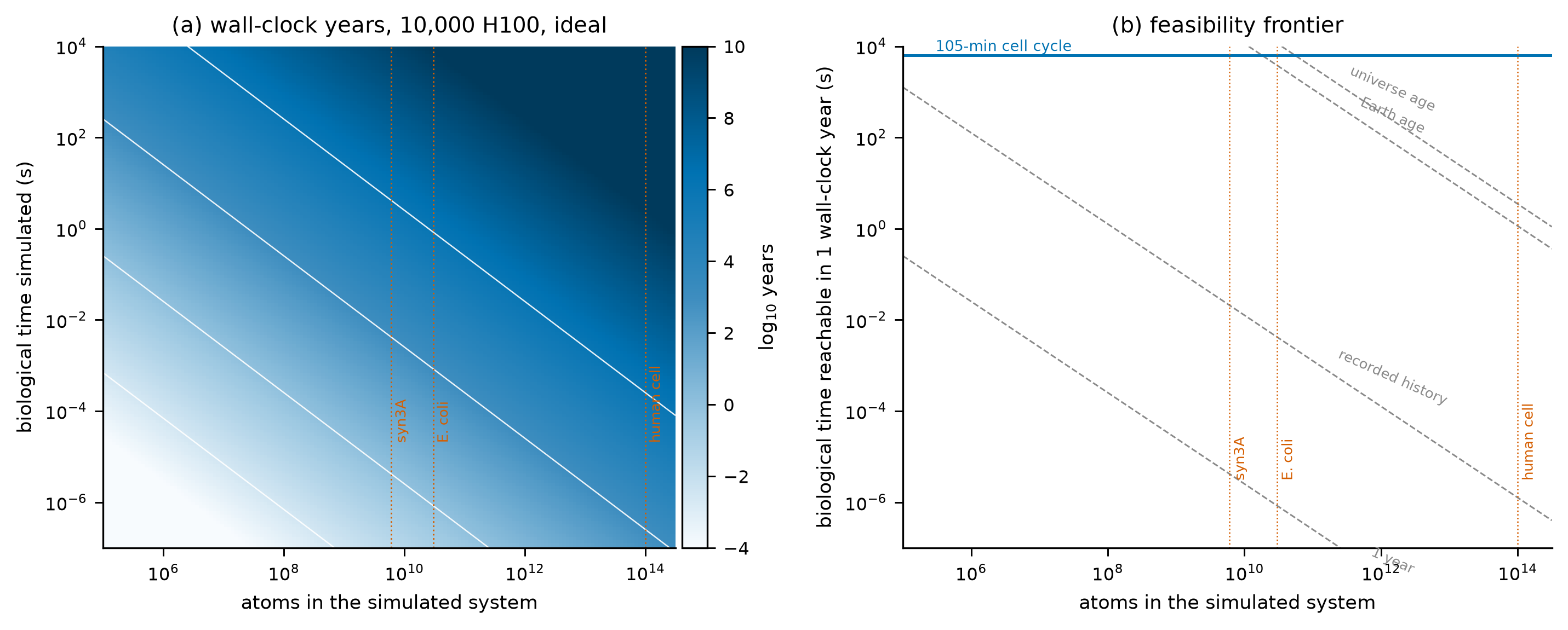
在”一万块 H100、理想弱扩展”这一乐观情景下，模拟 syn3A 全原子系统 1 秒需要约 24 万年，一个完整细胞周期约 15.0 亿年；大肠杆菌 1 小时约 42.8 亿年，人类细胞 1 小时约 14.3 万亿年。把 Anton 3 这样的专用机器放进同一张图，量级只下降一到两个数量级——因为原子数增加时，节点数不能无限增加。

Under the optimistic “10,000 H100, ideal weak scaling” scenario, one second of the all-atom syn3A system takes about 238 thousand years, and a full cell cycle about 1.5 billion years; one hour of E. coli about 4.3 billion years and one hour of a human cell about 14.3 trillion years. Putting a special-purpose machine such as Anton 3 on the same plot buys one to two orders of magnitude, not more — because node count cannot grow without bound as atom count does.

科学计数法会把这些数字变成一串没有重量的零。换成人类能理解的单位，它们是这样的：syn3A 全原子跑 1 秒，大约等于智人出现以来的全部时间（0.8 倍）；跑完一个细胞周期，大约是地球年龄的三分之一（0.33 倍）；大肠杆菌跑 1 小时，约等于地球的年龄（0.9 倍）；人类细胞跑 1 小时，约等于宇宙年龄的 1,030 倍。这不是”再等几代硬件”的量级，而是”从恐龙灭绝算起也跑不完一个细胞周期”的量级。

Scientific notation turns these numbers into a string of weightless zeros. In units a person can feel, they read like this: one second of all-atom syn3A is roughly the entire time since Homo sapiens appeared (0.8×); one cell cycle is about a third of the age of the Earth (0.33×); one hour of E. coli is about the age of the Earth (0.9×); one hour of a human cell is about 1,030 times the age of the universe. This is not a “wait a few hardware generations” scale; it is a “not even starting at the dinosaurs would finish one cell cycle” scale.

图 2　同样的计算，换成人类能理解的单位。(a) 四条彩线是四次模拟所需的墙钟年数（一万块理想 GPU）；下方五条灰线是自然时间尺度：人类文明、智人出现、恐龙灭绝、地球年龄、宇宙年龄。syn3A 一秒 ≈ 智人历史，一个细胞周期 ≈ 地球年龄的三分之一，大肠杆菌一小时 ≈ 地球年龄，人类细胞一小时 ≈ 宇宙年龄的一千倍。(b) 同一批计算的耗电量，以当前世界年用电量为单位：从 syn3A 一秒的 0.43 倍，到人类细胞一小时的 2,600 万倍。假设每块 GPU 300 W、世界年用电 29,000 TWh、理想弱扩展；能量只取决于总功，不随并行度改变。 | Figure 2. The same computation in units a person can feel. (a) The four coloured lines are wall-clock years for four simulations on 10,000 ideal GPUs; the five grey lines below are natural timescales: recorded history, Homo sapiens, the dinosaurs, the age of the Earth and the age of the universe. One second of syn3A ≈ human history, one cycle ≈ a third of Earth’s age, one hour of E. coli ≈ Earth’s age, one hour of a human cell ≈ a thousand universe ages. (b) Electricity for the same runs, in years of current world consumption: from 0.43× for one second of syn3A to 26 million× for one hour of a human cell. Assumes 300 W per GPU, 29,000 TWh per year, ideal weak scaling; energy depends only on total work and not on parallelism.

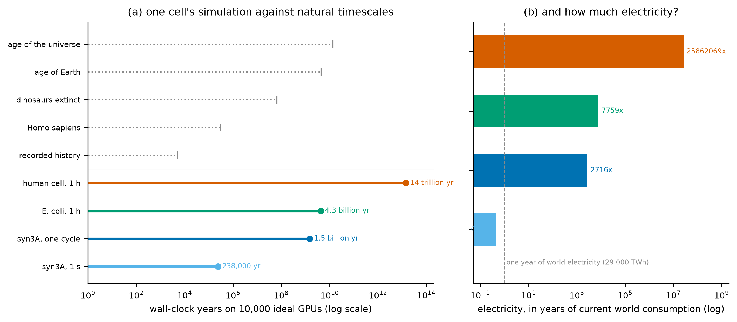
电量的账同样直白：按每块 GPU 300 W、当前世界年用电 29,000 TWh 计算，syn3A 跑 1 秒要烧掉 0.43 年的世界用电量，一个细胞周期要 2,716 年，大肠杆菌 1 小时要 7,759 年，人类细胞 1 小时要 26,000,000 年。换一个问法更刺人：如果要求在一个日历年内算完一个 syn3A 细胞周期，需要约 30 万亿块 GPU，总功率约 9,000 TW，是当前世界总发电功率的几百倍。时间、电量、机器数量，三个轴都指向同一个结论。

The electricity ledger is equally blunt. At 300 W per GPU and 29,000 TWh of world electricity per year, one second of syn3A burns 0.43 years of world electricity; one cycle burns 2,716 years; one hour of E. coli 7,759 years; one hour of a human cell 26,000,000 years. A sharper way to ask: to finish one syn3A cycle within a calendar year you would need about 30 trillion GPUs and roughly 9,000 TW of power, several hundred times the world’s total generating capacity. Time, electricity and machine count all point the same way.

图 3　(a) 不同硬件情景下，模拟 syn3A 与大肠杆菌各 1 小时所需的墙钟年数。顶部横轴标出 1 天、1 年、5 千年、45 亿年与 138 亿年作为参照。(b) 状态存储（每原子 150 字节）与 10⁴ 帧轨迹（每原子 12 字节）随原子数的增长，以及三种集群容量。 | Figure 3. (a) Wall-clock years for one hour of syn3A and of E. coli under several hardware scenarios; the top axis marks one day, one year, 5 kyr, 4.5 Gyr and 13.8 Gyr. (b) State storage (150 bytes per atom) and a 10⁴-frame trajectory (12 bytes per atom) against atom count, with three cluster capacities.

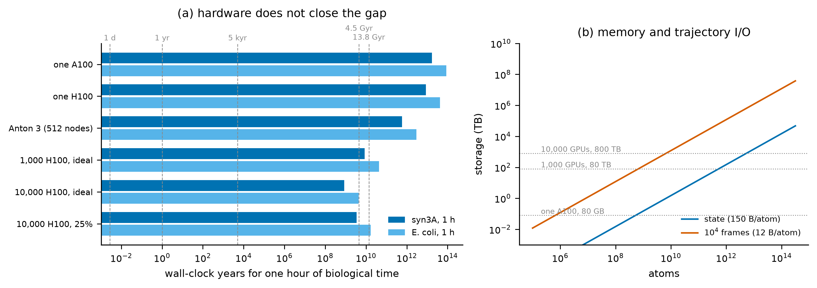
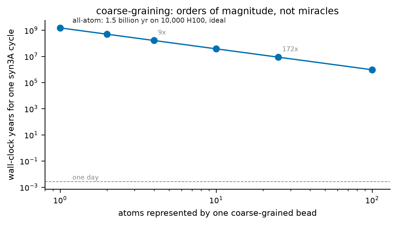
墙不只有时间。syn3A 的状态数组约 0.9 TB，还在一个集群的内存范围内；人类细胞约 15 PB，已经超过任何单机的内存，只能靠极端的分布式存储。轨迹更糟：每原子每帧 12 字节，10⁴ 帧就是 PB 到 EB 级 I/O。粗粒化能买回三个数量级：每 100 个原子一个珠子、步长放大 16 倍，总加速约 1585 倍，但把一个 syn3A 周期从 10⁹ 年降到 10⁶ 年，仍然不是可执行的时间。

The wall is not only time. The syn3A state array is about 0.9 TB, still within a cluster’s memory; a human cell is about 15 PB, beyond any single machine and requiring extreme distributed storage. Trajectories are worse: 12 bytes per atom per frame, so 10⁴ frames means PB-to-EB I/O. Coarse-graining buys three orders of magnitude — one bead per 100 atoms and a 16-fold larger step give about 1585× — but it takes one syn3A cycle from 10⁹ years to 10⁶ years, still not an executable duration.

图 4　粗粒化把”不可行”变成”仍然不可行”。纵轴是一个 syn3A 细胞周期所需的墙钟年数，横轴是一个珠子代表的原子数；灰虚线是一天。 | Figure 4. Coarse-graining turns “infeasible” into “still infeasible”. The vertical axis is wall-clock years for one syn3A cycle; the horizontal axis is the number of atoms per bead; the grey dashed line is one day.

必须把话说准：这不是逻辑上的不可能。短窗口的全原子模拟已经在进行：syn3A 的细胞质在微秒到毫秒尺度上有真实的全原子或近全原子研究，专门的 Anton 类机器也确实在推进可及的时间尺度。墙的位置取决于问题：如果你想问”这个突变在 10 微秒内如何改变一个活性位点”，答案是可行的；如果你想问”这个细胞在一个周期里如何决定命运”，全原子 MD 不是正确的工具。成本分析给出的不是禁令，而是分辨率与问题之间的匹配表。

Precision matters here: this is not a logical impossibility. Short windows of all-atom simulation are already done — the syn3A cytoplasm has been studied at microsecond-to-millisecond scales, and special-purpose machines such as Anton really do push the accessible timescale. The wall depends on the question: “how does this mutation change an active site within 10 µs” is feasible; “how does this cell decide its fate over a cycle” is not a question for all-atom MD. The cost analysis yields not a prohibition but a matching table between resolution and question.

还有两条常被用来推翻这张表的论据，值得单独检查。第一是机器学习势能：它把量子化学精度带到更大的体系，确实改变了”每个原子每秒”的成本，但它没有改变标度——一个神经网络势的每一步仍然要对每个原子做固定次数的运算，通信与内存带宽仍然是主要瓶颈。第二是”再等十年”：如果硬件每年快 1.5 倍，十年就是 57 倍，二十年是 3300 倍；而 syn3A 一个周期需要 10^9 年，人类细胞一小时需要 10^13 年。指数增长是真的，但差距的指数更大。 这不是说硬件无用；它说的是，把分辨率当成唯一的旋钮，收益会递减得很快。

Two arguments often used against this table deserve separate inspection. The first is machine-learned potentials: they bring quantum-chemical accuracy to larger systems and genuinely change the cost per atom per second, but they do not change the scaling — a neural-network potential still does a fixed amount of work per atom per step, and communication and memory bandwidth remain the bottlenecks. The second is “wait ten years”: if hardware improves 1.5-fold per year, ten years is 57× and twenty years 3,300×; one syn3A cycle needs 10⁹ years and one hour of a human cell 10¹³ years. Exponential growth is real, but the gap’s exponent is larger. This is not an argument that hardware is useless; it says that resolution as the only knob has rapidly diminishing returns.

3. 结构不决定状态 / Structure does not fix the state

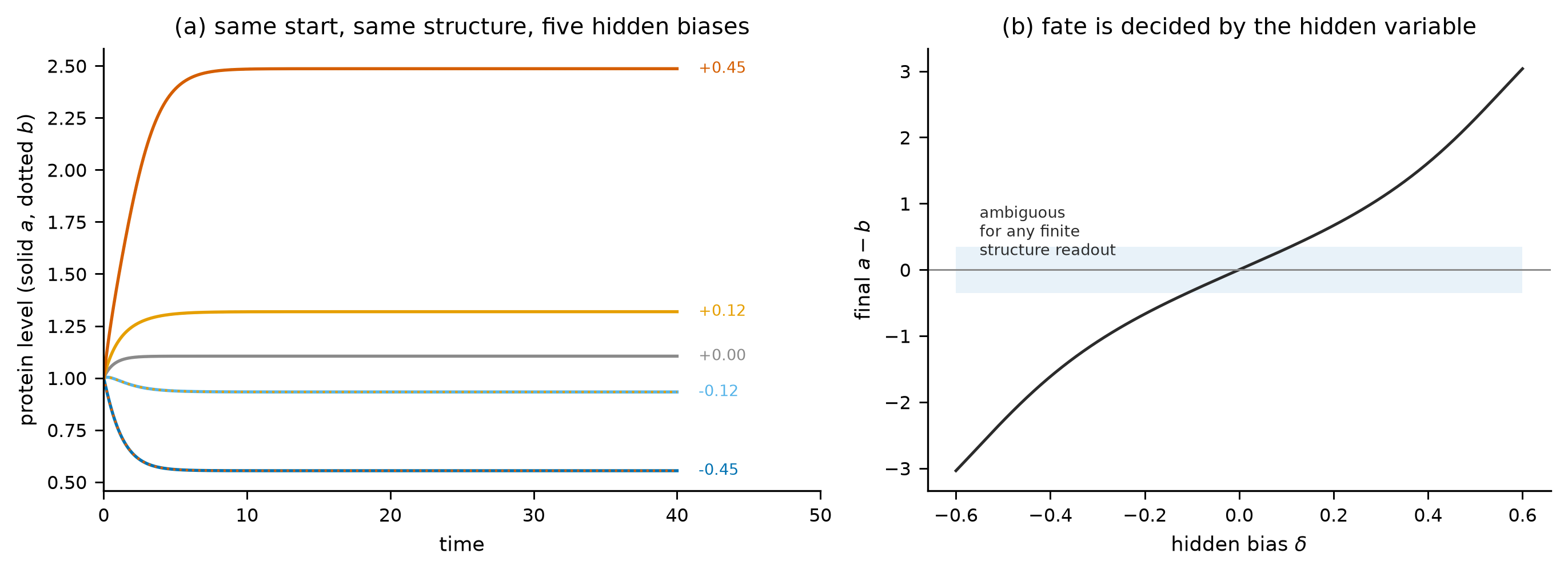
第二个问题更尖锐：即使算力无限，结构信息是否足以确定细胞的未来？我们把这个问题做成一个双稳态开关。两个基因互相抑制，隐藏变量 δ 是一个”染色质样”的偏置，决定哪一侧最终获胜；“结构读出”是 δ 的一个带噪、被压缩的测量。五个不同的 δ 从完全相同的初始蛋白水平出发，走向五种不同的命运。

The second question is sharper: even with unlimited compute, is structural information enough to determine a cell’s future? We make it concrete with a bistable toggle. Two genes inhibit each other; a hidden variable δ is a chromatin-like bias that decides which side wins; the “structure readout” is a noisy, compressed measurement of δ. Five values of δ start from exactly the same initial protein levels and end in five different fates.

图 5　(a) 相同的初始状态、相同的网络、相同的参数，只有隐藏偏置 δ 不同，最终命运分成两支。(b) 终点差值 \(a-b\) 随 δ 的变化；浅蓝色带是任何有限精度的结构读出都无法区分的区域。 | Figure 5. (a) Same initial state, same network, same parameters, only the hidden bias δ differs; the final fate splits in two. (b) Final \(a-b\) against δ; the pale band is the region no finite-precision structural readout can resolve.

在这个系统上，“知道结构”被操作化为”以噪声 σ_s 观测 δ”。最优解码器的贝叶斯错误率随 σ_s 上升：当 σ_s = 0.5 时，结构读出的贝叶斯错误率为 28.5%；把 RNA 读出加进来（σ 减半）降到 16.4%，再加染色质（σ 降到五分之一）降到 6.6%。信息论给出同一件事的另一种读数：命运本身的熵是 1.00 比特，结构读出只携带 0.78 比特，加上染色质后升到 0.93 比特——仍然小于 1。数据处理不等式在这里不是一个比喻：它是可算的上界。

“Knowing the structure” is operationalised as observing δ with noise σ_s. The Bayes error of the optimal decoder rises with σ_s: at σ_s = 0.5 the structural readout has a Bayes error of 28.5%; adding an RNA readout (halving σ) lowers it to 16.4%, and adding chromatin (σ/5) to 6.6%. Information theory gives another reading of the same fact: the entropy of the fate itself is 1.00 bits, the structural readout carries 0.78 bits, and adding chromatin raises it to 0.93 bits — still below one. The data-processing inequality is not a metaphor here; it is a computable bound.

图 6　(a) 贝叶斯错误率随读出噪声的变化；三条曲线对应三种观测组合。(b) 给定读出后，未来状态 \(a_T\) 的条件标准差随预测视界增长，最终饱和到由读出精度决定的条件值；灰虚线是无读出时的先验标准差，两者之间的差距就是读出买到的信息。短视界看起来”可辨识”，是因为还没到分岔。(c) 熵与互信息：结构读出不足以覆盖命运的全部不确定性。 | Figure 6. (a) Bayes error against readout noise for three observation sets. (b) The conditional standard deviation of the future state \(a_T\) grows with the horizon and saturates at a value set by readout precision; the grey dashed line is the prior without any readout, and the gap is what the readout buys. Short horizons look identifiable because the bifurcation has not happened yet. (c) Entropy and mutual information: the structural readout does not cover the uncertainty of the fate.

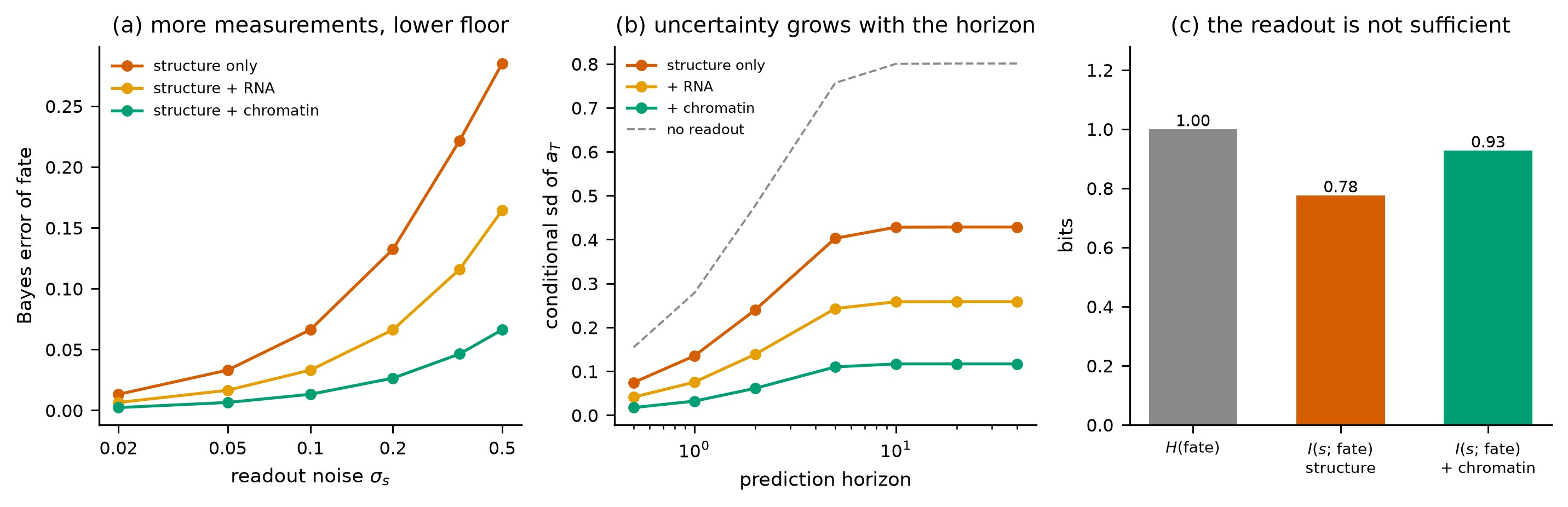
由此可以陈述一个有条件的命题，而不是一个口号：若 (i) 存在至少两个隐藏状态在给定结构读出下不可区分，(ii) 这两个隐藏状态导致不同的未来表型，(iii) 读出噪声有下界，则任何仅以结构为输入的确定性预测器，其最坏情况误差有非零下界；任何随机预测器的贝叶斯风险不低于该下界。这个命题不排斥概率预测：它恰恰说明概率预测是必要的。它也不排斥”更多测量”：加染色质就把界降低了。它排斥的是一种特定的自信——“有了结构，剩下的只是算”。

One can therefore state a conditional proposition rather than a slogan: if (i) at least two hidden states are indistinguishable under the structural readout, (ii) they lead to different future phenotypes, and (iii) the readout noise is bounded below, then any deterministic predictor using only structure has a non-zero worst-case error, and any stochastic predictor has Bayes risk above that bound. The proposition does not rule out probabilistic prediction — it makes it necessary. Nor does it rule out more measurements: adding chromatin lowers the bound. What it rules out is a particular kind of confidence — “with the structure in hand, only arithmetic remains”.

这些隐藏状态在真实细胞里有具体的名字：启动子区的染色质可及性、mRNA 的亚细胞定位、蛋白的磷酸化状态、细胞周期相位、以及细胞在组织中的位置。它们中的每一个都可以在”蛋白质组相同”的细胞之间不同，而每一个都可能改变同一扰动下的响应。更麻烦的是，它们往往互相耦合：染色质状态影响转录bursting，bursting影响蛋白水平，蛋白水平又通过反馈影响染色质。这就是为什么”结构 + 浓度”的快照不足以定义初始条件，而不是因为测量还不够精确。

These hidden states have concrete names in real cells: chromatin accessibility at promoters, subcellular localisation of mRNA, phosphorylation state of proteins, cell-cycle phase, and position within a tissue. Each can differ between cells with the same proteome, and each can change the response to the same perturbation. Worse, they are coupled: chromatin state affects transcriptional bursting, bursting affects protein levels, and protein levels feed back on chromatin. That is why a snapshot of “structure plus concentrations” does not define the initial condition — not because the measurement is not precise enough.

4. 封闭性：记忆从哪里来 / Closure: where memory comes from

假设我们把状态测量全了。下一个问题是：能不能把它压缩，仍然得到一个只依赖当前粗粒状态的方程？这就是 Mori–Zwanzig 的问题。我们用一个十维线性系统做精确实验：两个慢变量、八个快变量，快变量是阻尼旋转，因此记忆核会振荡着衰减。线性系统的记忆核可以精确写出：\(K(\tau)=A_{sf}e^{A_{ff}\tau}A_{fs}\)。

Suppose the state is fully measured. The next question is whether it can be compressed into an equation that depends only on the current coarse state. That is the Mori–Zwanzig question. We run an exact experiment on a ten-dimensional linear system: two slow variables, eight fast ones, with the fast block built from damped rotations so that the memory kernel oscillates as it decays. For a linear system the kernel is exact: \(K(\tau)=A_{sf}e^{A_{ff}\tau}A_{fs}\).

图 7　(a) 记忆核的范数随滞后时间衰减，衰减时间由快时间尺度决定。(b) ε = 0.5 时三种约化模型的相对误差随时间的变化：马尔可夫闭合缺失记忆，AR(2) 只是部分补偿，带记忆核的模型误差低两个数量级。(c) 闭合误差随时间尺度分离 ε 的变化；马尔可夫误差从 1.1e-04 升到 0.158，拟合斜率约 1.65；记忆模型的误差保持在 0.0043 附近，那是数值积分偏差，不是模型误差。 | Figure 7. (a) The norm of the memory kernel decays on the fast timescale. (b) Relative error of three reduced models against time at ε = 0.5: the Markov closure misses memory, AR(2) only partly compensates, and the memory model is two orders of magnitude better. (c) Closure error against the timescale separation ε; the Markov error rises from 1.1e-04 to 0.158 with a fitted slope near 1.65, while the memory model stays near 0.0043, which is quadrature bias rather than model error.

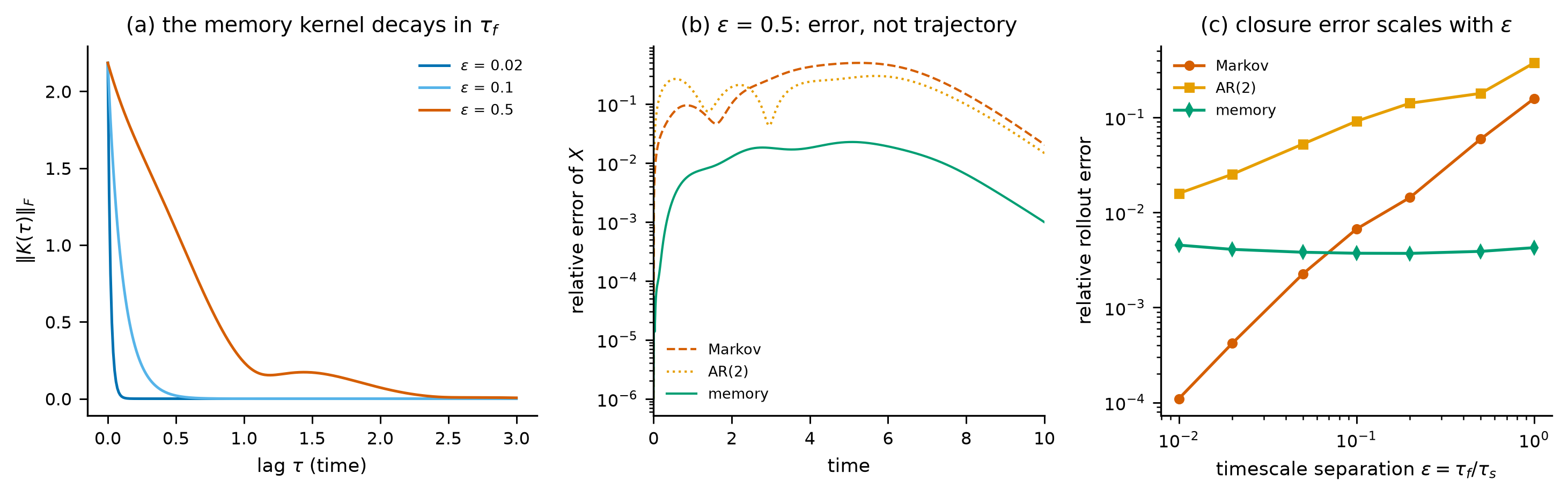
这张图要避免一个常见的误读。Mori–Zwanzig 并没有”证明所有粗粒化都会失败”；它给出的是精确的广义朗之万方程，只是方程里多了一个记忆积分。失败的是”把记忆丢掉”这个近似，而近似的误差有明确的条件：当 ε = τ_fast/τ_slow 很小时，马尔可夫闭合几乎正确（ε = 0.01 时误差 1.1e-04）；当 ε 接近 1，误差升到 0.158，与 ε 近似同阶。所以正确的说法是：封闭性不是免费的，它的价格是 ε；如果系统里存在几个不比慢变量快多少的中间尺度，价格就会很贵。

One misreading must be blocked. Mori–Zwanzig does not “prove that all coarse-graining fails”; it gives an exact generalised Langevin equation, with a memory integral added. What fails is the approximation that drops memory, and its error has a clear condition: for small ε = τ_fast/τ_slow the Markov closure is almost exact (error 1.1e-04 at ε = 0.01); as ε approaches one the error rises to 0.158, roughly linear in ε. The right statement is: closure is not free; its price is ε, and that price is high when intermediate timescales sit close to the slow ones.

形式化地说，投影算子把状态分成”保留的”与”被消去的”两部分，把后者对前者的影响写成两件事：一个瞬时的平均力，以及一个对历史的卷积记忆；再外加一项由初始条件决定的”残余”。前两项是确定性的，第三项在热浴极限下变成噪声，而噪声的强度由涨落—耗散关系与记忆核绑定。这也解释了为什么”随机约化模型”不是一个独立的第五个模型：在线性高斯情形，它就是记忆模型加上与同一个核绑定的噪声，均值轨迹与记忆模型相同。本文因此没有把它单独画进图 7，否则会把同一条误差画两遍；代价是这篇文章少了一张图，收益是读者不会被两条重合的曲线误导。

Formally, a projection operator splits the state into a kept part and an eliminated part, and writes the influence of the latter on the former as three things: an instantaneous average force, a convolution over history, and a residual fixed by the initial condition. The first two are deterministic; in the heat-bath limit the third becomes noise, with its strength tied to the kernel by a fluctuation–dissipation relation. This is also why a “stochastic reduced model” is not an independent fifth model: in the linear-Gaussian case it is the memory model plus noise tied to the same kernel, with the same mean trajectory. It is therefore not drawn separately in Figure 7, which would plot the same error twice; the cost is one fewer panel, the benefit is not misleading the reader with two identical curves.

5. 浓度看不见通量 / Concentrations cannot see fluxes

生命是开放系统。一个三状态循环，外加一个化学势差驱动，局部细致平衡固定每条边正反向速率之比，整圈的亲和势为 \(A/k_BT\)。这个模型有一个漂亮的性质：对称循环的稳态分布对任何驱动都是均匀的，所以浓度快照完全不包含驱动的信息，而净通量与熵产生率包含。

Life is an open system. Take a three-state cycle driven by a chemical-potential difference; local detailed balance fixes the forward/backward ratio on every edge, and the affinity around the cycle is \(A/k_BT\). The model has a nice property: for the symmetric cycle the steady-state distribution is uniform at every drive, so a snapshot of concentrations carries no information about the drive, while the net flux and the entropy production rate do.

图 8　(a) 驱动同时买到通量与耗散：净通量 \(J\) 与熵产生率 \(\sigma\) 随亲和势上升，平衡点两者均为零。(b) 把网络的所有速率同乘 1、5、25 倍，稳态浓度完全不变（\(p_1=1/3\)），通量与熵产生率却按相同倍数变化（\(\sigma\) 从 1.9 到 47.8）。 | Figure 8. (a) Drive buys both flux and dissipation: net flux \(J\) and entropy production \(\sigma\) rise with affinity, and both vanish at equilibrium. (b) Scaling every rate by 1, 5 and 25 leaves the steady-state concentrations identical (\(p_1=1/3\)) while flux and entropy production scale with it (\(\sigma\) from 1.9 to 47.8).

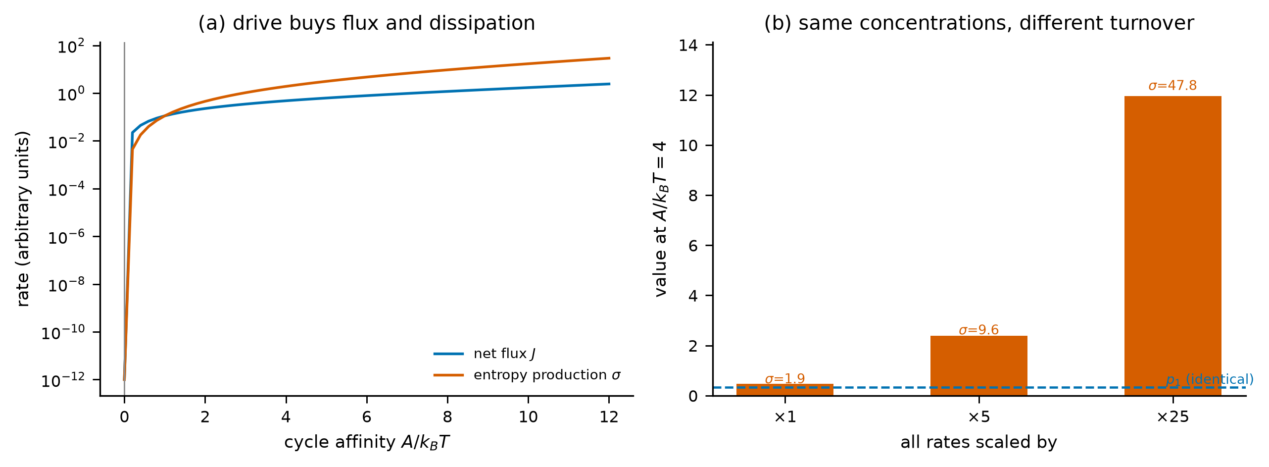
随机版本给出同一结论的另一个侧面。用精确 Gillespie 模拟跑 300 个时间单位，平衡系统（A = 0）的净顺时针圈数平均为 2.0，驱动系统（A = 4）为 142.7，与确定性预测 143.4 一致，标准差 7.8。两个系统的浓度分布一样，圈数分布完全不同。

The stochastic version shows another face of the same fact. In exact Gillespie runs of 300 time units, the equilibrium system (A = 0) winds 2.0 net clockwise cycles on average, the driven one (A = 4) 142.7, matching the deterministic prediction of 143.4 with a standard deviation of 7.8. The two systems have the same concentration distribution and completely different winding distributions.

图 9　(a) 平衡与驱动各一条随机轨迹；状态在三个节点间跳动，但只有驱动系统有净方向。(b) 固定时间内净顺时针圈数的分布：平衡系统中心在 0，驱动系统中心在 143 附近。 | Figure 9. (a) One stochastic trajectory each for equilibrium and drive; the state hops among three nodes, but only the driven system has a net direction. (b) Distribution of net clockwise windings in a fixed time: centred on zero at equilibrium and near 143 under drive.

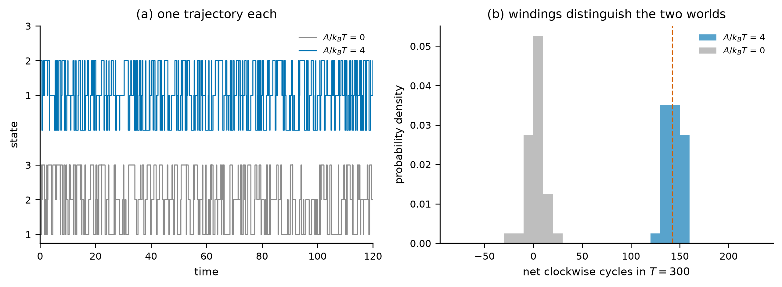
这解释了为什么”静态分子结构 + 浓度”不足以确定非平衡行为：结构给出的是可能的反应图，浓度给出的是节点占据率，而通量、熵产生率与驱动条件是第三层信息，只有在时间序列或扰动响应里才出现。热力学在这里的作用不是增加一个哲学维度，而是提供一个可测的量：σ 可以通过热耗散测量，圈数可以通过单分子追踪测量。

This explains why “static structure plus concentrations” cannot fix non-equilibrium behaviour: structure gives the possible reaction graph, concentrations give node occupancies, but flux, entropy production and the driving condition are a third layer that only appears in time series or perturbation responses. Thermodynamics adds not a philosophical dimension but a measurable quantity: σ can be estimated from heat dissipation, and windings from single-molecule tracking.

单位与适用条件必须写清楚。本文取 \(k_B=1\)，因此熵产生率的单位是”每单位时间的自然单位”，通量的单位是”每单位时间”；代入真实的速率常数后，\(\sigma\) 的单位是 \(k_B\,\mathrm{s^{-1}}\)，乘上 \(T\) 就是热耗散功率。这里的推导用了局部细致平衡（每条边的正反向速率比等于该边的自由能差），这对稀溶液中的基元反应是标准假设，但对有酶参与、有构象记忆的步骤未必成立；在那种情况下，网络热力学的”表观亲和势”可能依赖于速率常数的测量方式。这不是本文的模型能回答的问题，但它提醒读者：\(\sigma\) 是一个模型量，不是一台仪器直接读出的数。

Units and conditions must be stated. Throughout, \(k_B=1\), so entropy production is in natural units per unit time and flux is per unit time; with real rate constants, σ is in \(k_B\,\mathrm{s^{-1}}\), and multiplying by \(T\) gives dissipated power. The derivation assumes local detailed balance (the forward/backward ratio on each edge equals its free-energy difference), which is standard for elementary reactions in dilute solution but not guaranteed for enzyme-catalysed steps with conformational memory; there, the “apparent affinity” of network thermodynamics can depend on how rate constants are measured. This model cannot settle that question, but it is a reminder that σ is a model quantity, not a dial an instrument reads directly.

6. 分岔与噪声 / Bifurcations and noise

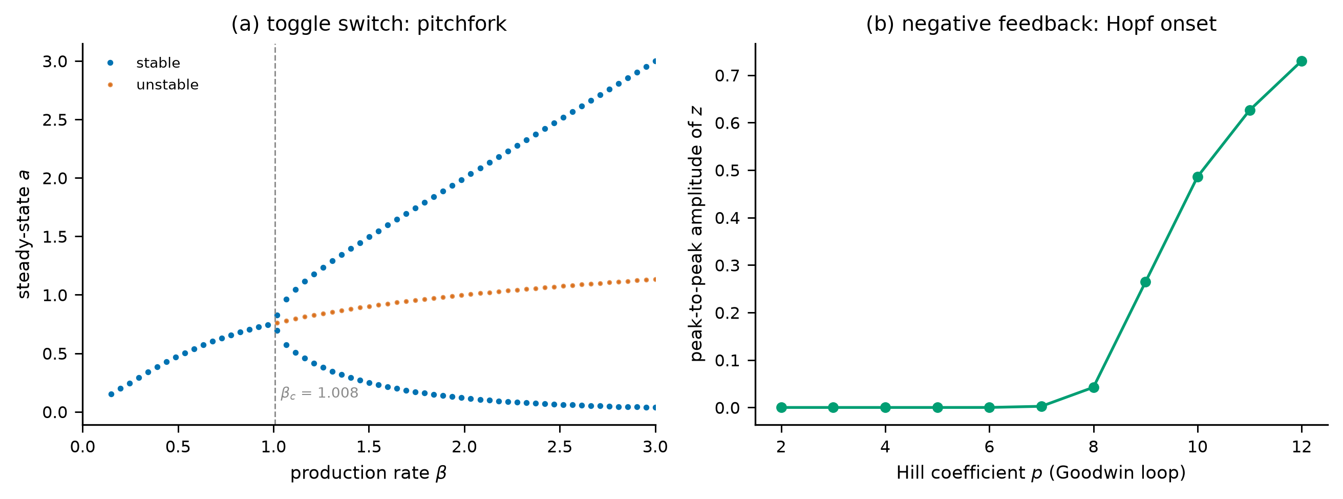
同一个网络、同一组参数，也可能有多个稳定状态。对称双稳态开关在 \(\beta_c = 1.008\) 处发生叉式分岔：低于它只有一个稳定点，高于它有两个。一个带负反馈的三节点 Goodwin 环路在 Hill 系数约 8 处发生 Hopf 分岔，从稳定焦点变成极限环。

The same network with the same parameters can also have several stable states. A symmetric toggle switch undergoes a pitchfork at \(\beta_c = 1.008\): below it there is one stable point, above it two. A three-node Goodwin loop with negative feedback undergoes a Hopf bifurcation near a Hill coefficient of 8, turning a stable focus into a limit cycle.

图 10　(a) 双稳态开关的分岔图：蓝点是稳定分支，红点是失稳的对称分支，虚线是 \(\beta_c = 1.008\)。(b) Goodwin 环路的极限环振幅随 Hill 系数变化，约在 p = 8 处起振。 | Figure 10. (a) Bifurcation diagram of the toggle switch: blue points are stable branches, red points the unstable symmetric branch, the dashed line is \(\beta_c = 1.008\). (b) Limit-cycle amplitude of the Goodwin loop against the Hill coefficient, with onset near p = 8.

把噪声加回来，命运就变成概率。在临界点附近，切换速率最高（\(\beta/\beta_c = 1.0\) 时 Ω = 40 的系统每单位时间 1.5e-02 次），随着系统尺寸增大而下降（Ω = 320 时观测不到切换）；远离临界点（\(\beta/\beta_c = 1.5\)）时切换几乎停止。

Put noise back and fate becomes a probability. Near the critical point the switching rate is highest (1.5e-02 per unit time at \(\beta/\beta_c = 1.0\) with Ω = 40) and falls as the system size grows (no transition observed at Ω = 320); far from criticality (\(\beta/\beta_c = 1.5\)) switching almost stops.

图 11　(a) Ω = 160 时的两条随机轨迹：\(\beta/\beta_c\) = 0.9 的系统在一个浅坑里抖动，1.08 的系统在两个坑之间来回切换。(b) 不同驱动下的 \(x-y\) 分布：一个峰或两个峰。(c) 切换速率随 (β, Ω) 的变化；白色表示在模拟时间内没有观测到切换。 | Figure 11. (a) Two stochastic trajectories at Ω = 160: the system at \(\beta/\beta_c\) = 0.9 fluctuates in one shallow well, while 1.08 switches between two. (b) Distribution of \(x-y\) at three drives: one peak or two. (c) Switching rate over (β, Ω); white marks no transition observed within the simulated time.

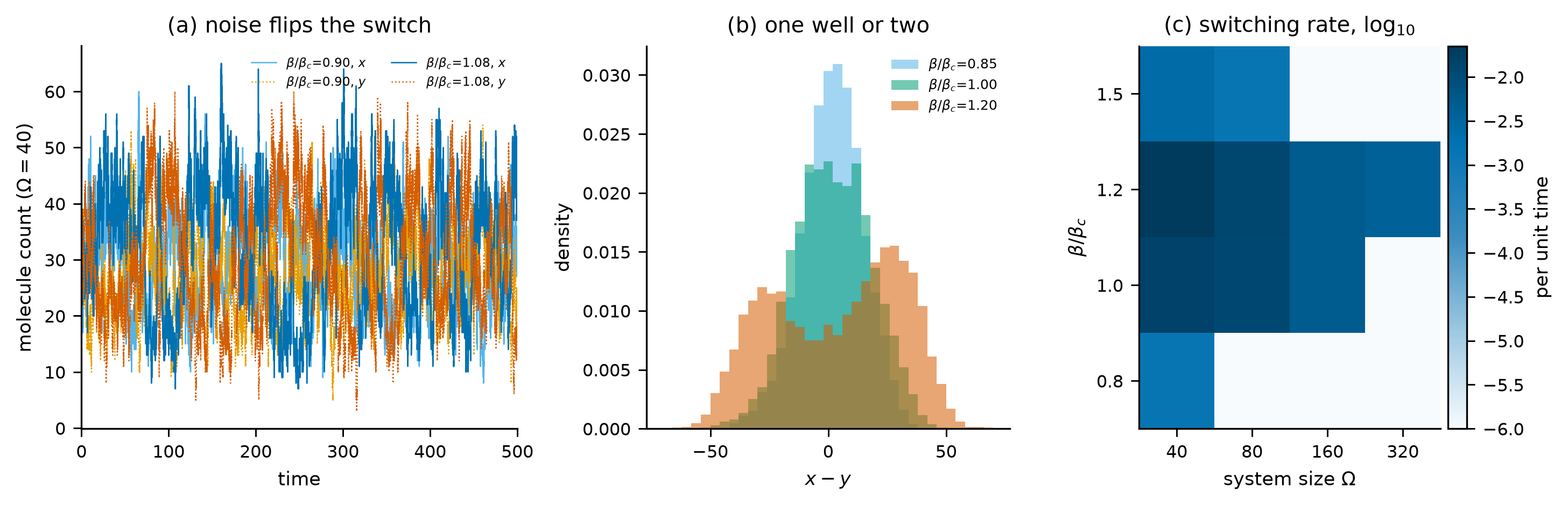
这一节的意义不是”噪声很重要”，而是它给出了敏感性的地图：在临界点附近，参数、初始条件与噪声的微小差异都会被放大成命运差异；在远离临界点的区域，同样的差异被系统的稳定性吸收。任何”平均细胞”模型都会在这张地图的红色区域失效，因为平均恰好抹掉了决定命运的那一维。

The point is not “noise matters” but that this gives a map of sensitivity: near criticality, small differences in parameters, initial conditions and noise are amplified into different fates; away from it, the same differences are absorbed by stability. Any “average cell” model fails in the red region of that map, because averaging erases exactly the dimension that decides the fate.

临界点附近还有一个可测的副产品：临界慢化。系统越接近分岔，恢复速率越慢，自相关时间越长；这在图 11(a) 里表现为 \(\beta/\beta_c = 1.08\) 的轨迹在两个坑之间停留的时间远长于坑内的抖动时间。对实验而言，这意味着”响应变慢”本身可以是一个前兆信号——不需要看到命运分叉，只要测量恢复时间就能判断系统离临界点有多近。这也给虚拟细胞一个可操作的检验：如果模型预测某个细胞群体处在临界点附近，它应当同时预测恢复时间的延长；如果只预测命运比例而不预测动力学，它就没有用上这个信息。

Near criticality there is a measurable by-product: critical slowing down. The closer the system is to the bifurcation, the slower the recovery and the longer the autocorrelation time; in Figure 11a this shows up as the \(\beta/\beta_c = 1.08\) trajectory dwelling far longer between wells than within one. For experiments this means that “slowing down” can itself be an early warning — one need not see the fate split to estimate how close the system is to criticality, only measure the recovery time. This gives a virtual cell an operational test: if the model says a population sits near a critical point, it should also predict longer recovery times; a model that predicts only fate fractions and not dynamics has not used that information.

7. 误差如何长成表型 / How error becomes phenotype

分子层的误差不是抽象的不确定性，它有单位。结合自由能的误差通过 \(K_d=\exp(\Delta G/RT)\) 指数放大：室温下 \(RT=0.592\) kcal/mol，1 kcal/mol 的误差就是 \(K_d\) 上 5.4 倍的误差。把这一层接上一个三级 Hill 级联和一个命运阈值，就得到误差传播的完整链条。

Error at the molecular level is not abstract uncertainty; it has units. A binding free-energy error is amplified exponentially through \(K_d=\exp(\Delta G/RT)\): at room temperature \(RT=0.592\) kcal/mol, so a 1 kcal/mol error is a factor 5.4 in \(K_d\). Connecting this layer to a three-tier Hill cascade and a fate threshold gives the full error-propagation chain.

图 12　(a) 自由能到平衡常数是指数映射，浅色带是 ±0.5 与 ±1 kcal/mol。(b) 两种工作点：饱和、带负反馈的级联几乎不受影响；靠近阈值的级联在同一误差下走完整条 S 曲线。(c) 蒙特卡洛传播：σ_ΔG = 1 kcal/mol 时，缓冲区的表型标准差为 0.000，临界区为 0.327；2 kcal/mol 时分别为 0.142 与 0.431。(d) 一阶 Sobol 指数：缓冲区由阈值 τ 主导（0.71），临界区由 \(K_1\) 与 ΔG 主导。 | Figure 12. (a) Free energy maps exponentially onto the equilibrium constant; shaded bands are ±0.5 and ±1 kcal/mol. (b) Two operating points: a saturated cascade with negative feedback is almost unaffected, while a cascade near threshold traverses the whole S-curve under the same error. (c) Monte Carlo propagation: at σ_ΔG = 1 kcal/mol the phenotype sd is 0.000 in the buffered regime and 0.327 near threshold; at 2 kcal/mol they are 0.142 and 0.431. (d) First-order Sobol indices: the buffered regime is dominated by the threshold τ (0.71), the critical one by \(K_1\) and ΔG.

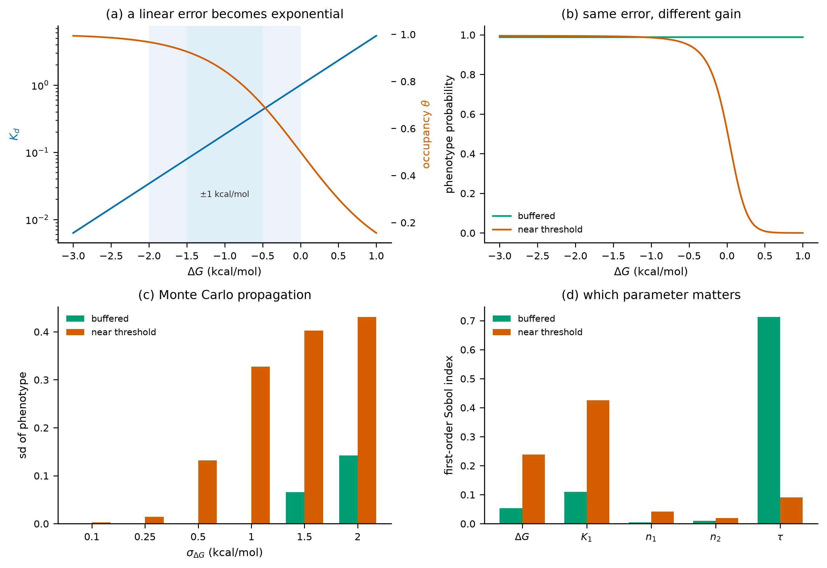
结论必须是有条件的：误差不一定被放大，放大与否取决于工作点。 饱和级联把误差压到零，但代价是它对阈值 τ 极其敏感——Sobol 指数 0.71 说明” robust “只是把脆弱性换了一个位置。临界区把误差放大到表型分布的另一端，但它对 ΔG 的敏感性也更接近物理直觉。这对虚拟细胞是一个直接的要求：报告一个预测时，必须同时报告它处在参数空间的哪个区域。

The conclusion has to be conditional: error is not always amplified; amplification depends on the operating point. The saturated cascade suppresses it, but at the price of extreme sensitivity to the threshold τ — a Sobol index of 0.71 says that “robust” only moved the fragility elsewhere. The critical regime amplifies error into the tails of the phenotype distribution, but its sensitivity to ΔG is closer to physical intuition. For a virtual cell this is a direct requirement: a prediction must come with the region of parameter space it lives in.

这里需要区分两种误差，它们的处理方式完全不同。参数误差是方程对了、常数错了：可以靠更多数据、更好的拟合或贝叶斯先验来缩小，第 9 节的”参数错 15%“就是这一类。结构误差是方程本身错了：比如用零维模型描述一个有空间结构的系统（第 8 节），或用一个不含记忆的方程描述一个 ε 接近 1 的系统（第 4 节）。结构误差不能被参数拟合消除，只会被参数拟合掩盖——你会得到一组”看起来能拟合训练数据”的参数，然后在新的扰动下失败。这也是为什么本文把第 8、9 节的反例放在一起：它们分别说明结构误差与参数误差，而虚拟细胞的很多失败案例，是把结构误差误诊成了参数误差。

Two kinds of error must be distinguished, because they are handled differently. Parameter error means the equations are right and the constants are wrong: it can be reduced with more data, better fitting or Bayesian priors, and the “15% parameter error” of Section 9 is of this kind. Structural error means the equations themselves are wrong: for example a zero-dimensional model describing a spatially structured system (Section 8), or a memoryless equation describing a system with ε near one (Section 4). Structural error cannot be removed by fitting parameters; it is only masked by them — one obtains parameters that fit the training data and then fails under a new perturbation. That is why the counterexamples of Sections 8 and 9 belong together: they illustrate structural and parameter error respectively, and many failures of virtual cells are structural errors misdiagnosed as parameter errors.

8. 空间：烧瓶何时失效 / When the flask fails

到目前为止所有模型都是充分混合的。真实细胞不是。我们用一个双稳态反应扩散系统检验”同样的分子总量、不同的空间分布”是否等价：一个总量固定为 15 的高斯源，σ 从 2 变到 12，铺在 96×96 的格子上，反应项是双稳态的 Schlögl 型。

So far every model has been well mixed. Real cells are not. We test whether “the same total amount, differently distributed” is equivalent, using a bistable reaction–diffusion system: a Gaussian source of fixed total mass 15, with σ from 2 to 12, on a 96×96 grid, with a bistable Schlögl-type reaction term.

图 13　同一总量、不同宽度的局部输入。上行是窄源（σ = 3）：局部点燃后保持一个高态区域；下行是宽源（σ = 10）：峰值低于点火阈值，什么也没有发生。 | Figure 13. The same total input at different widths. Top: a narrow source (σ = 3) ignites locally and keeps a high-state region. Bottom: a broad source (σ = 10) has a peak below the ignition threshold and nothing happens.

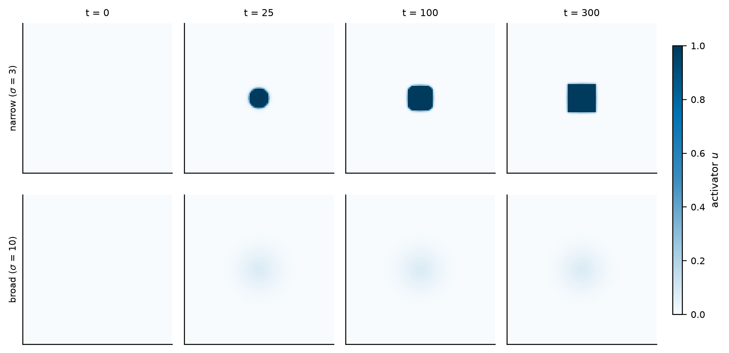
演化动画：σ = 3 的窄源从零态点燃并扩张。 / Animation: the narrow σ = 3 source ignites from the low state and spreads.

定量结果很干净：σ = 3 时高态占 3.5%，σ = 10 时高态占 0.0%；而任何只看到总量（平均输入 15/96²）的零维模型都预测 0.0%。点火阈值在 σ ≈ 9 处：峰值跌破阈值，整个响应消失。

The numbers are clean: at σ = 3 the high state covers 3.5% of the domain, at σ = 10 0.0%; any zero-dimensional model that sees only the total (mean input 15/96²) predicts 0.0%. The ignition threshold sits near σ ≈ 9: the peak falls below it and the response disappears.

图 14　(a) 高态比例随 Damköhler 数（σ²/D）的变化；零维模型（虚线）对所有几何给出同一个错误答案。(b) 三个宽度的时间过程：点火是全或无的。(c) 烧瓶近似的适用条件：当衰减长度 λ 远大于细胞尺度 L 时，核内响应接近混合预测；λ = L 时只剩 64.8%，而不是 97.4%。 | Figure 14. (a) High-state fraction against the Damköhler number (σ²/D); the zero-dimensional model (dashed) gives the same wrong answer for every geometry. (b) Time courses for three widths: ignition is all-or-none. (c) When the flask approximation holds: for a decay length λ much larger than the cell size L the nuclear response approaches the well-mixed prediction; at λ = L it is only 64.8% instead of 97.4%.

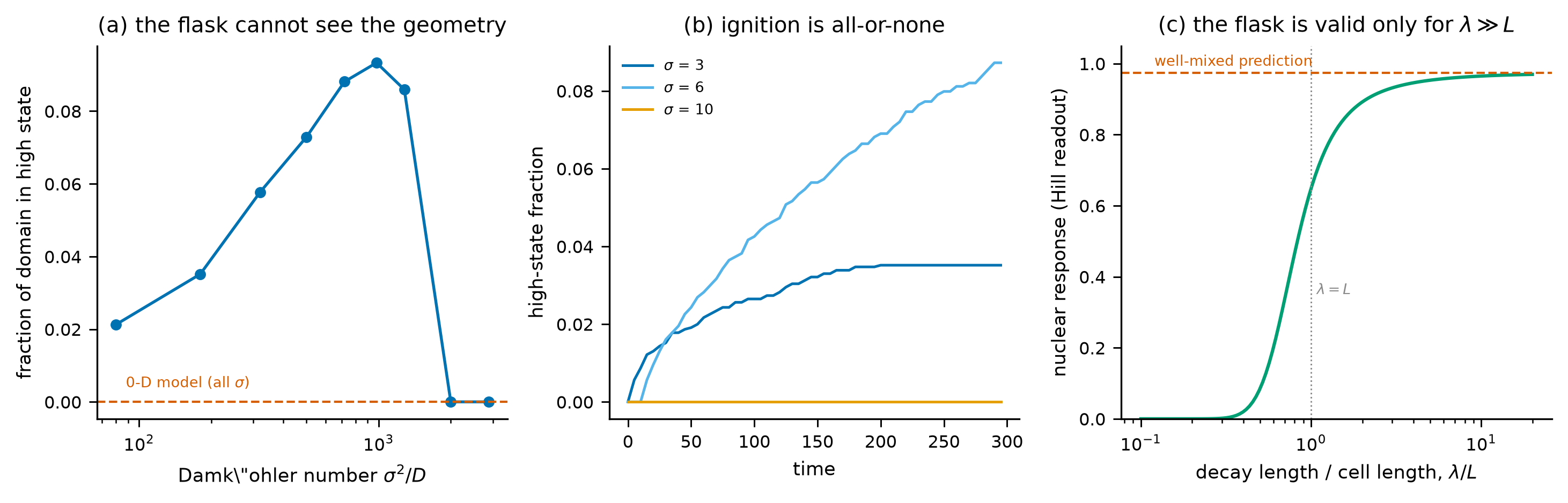
因此”充分混合”不是一个可以默认的近似，而是一个有条件的近似：当 Damköhler 数小、或衰减长度远大于细胞尺度时成立。反过来，只要信号在空间上有结构，烧瓶就会系统性地错。这个结论对虚拟细胞尤其重要，因为大多数单细胞模型都是零维的。

So “well mixed” is not a default approximation but a conditional one: it holds when the Damköhler number is small, or when the decay length is much larger than the cell. Conversely, whenever the signal has spatial structure, the flask is systematically wrong. This matters for virtual cells, most of which are zero-dimensional.

为什么大多数细胞模型仍然是零维的？因为零维模型容易标定、容易与组学数据对齐，而且在”平均行为”上往往够用。问题在于，“平均行为够用”本身是一个需要证明的命题，而不是一个默认设置。 第 8 节的判据给出了一个廉价的检验：估计信号的衰减长度 λ 与细胞尺度 L 的比值；如果 λ/L 大于几，零维近似安全；如果接近或小于 1，就必须引入空间。这个检验不需要解 PDE，只需要一个扩散系数与一个降解速率。把这样的判据写进建模流程，比事后解释”为什么空间模型更好”要有效得多。

Why are most cell models still zero-dimensional? Because zero-dimensional models are easy to calibrate, easy to align with omics data, and often adequate for “average behaviour”. The problem is that “adequate for average behaviour” is a proposition to be proved, not a default setting. Section 8 supplies a cheap test: estimate the ratio of the signal’s decay length λ to the cell size L; if λ/L is several, the zero-dimensional approximation is safe; if it is near or below one, space must enter. The test needs no PDE solve, only a diffusion coefficient and a degradation rate. Writing such a criterion into the modelling workflow is far more effective than explaining afterwards why the spatial model did better.

9. 分辨率与预测 / Resolution and prediction

现在把所有线索收进一个比较：六个模型，同一批初始条件，同一个”细胞”（十二维、六慢六快），同一个表型。它们的信息量与成本刻意做成阶梯：精确参数的细模型、参数错 15% 的细模型、把快变量放在准稳态的粗模型、数据拟合的线性 VAR、直接从初态映射到表型的 MLP、粗模型加学习残差的混合模型，以及只知道网络、不知道状态的”结构模型”。

Now collect the threads into one comparison: six models, the same initial conditions, the same “cell” (twelve variables, six slow and six fast), the same phenotype. Information and cost form a deliberate ladder: a fine model with exact parameters, the same with 15% parameter error, a coarse model with the fast subsystem at quasi-steady state, a fitted linear VAR, an MLP mapping the initial state directly to phenotype, a hybrid of coarse simulation plus a learned residual, and a “structure” model that knows the network but not the state.

图 15　(a) 误差—成本平面（对数轴；成本是 400 次预测的墙钟秒数，包含训练）。细模型最准但最贵；参数错 15% 的细模型比粗模型更差，是最直接的负面结果；混合模型以细模型约十分之一的成本达到粗模型的精度。(b) 状态观测与参数精度的交互：只观测一两个慢变量时，四条曲线都停在表型方差附近，参数精度无处施展；六个状态全部观测后，误差才随参数误差从 3.6e-05 升到 0.161。(c) 学习型修正的误差随训练轨迹数下降。 | Figure 15. (a) The error–cost plane (log axes; cost is wall-clock seconds for 400 predictions, fitting included). The fine model is most accurate and most expensive; the fine model with 15% parameter error is worse than the coarse one, the most direct negative result here; the hybrid reaches the coarse model’s accuracy at about a tenth of the fine model’s cost. (b) State observation interacts with parameter precision: with only one or two slow variables observed, all four curves sit near the phenotype variance and precision has nowhere to act; only after all six are observed does the error fall with parameter error, from 3.6e-05 to 0.161. (c) The learned correction improves with the number of training trajectories.

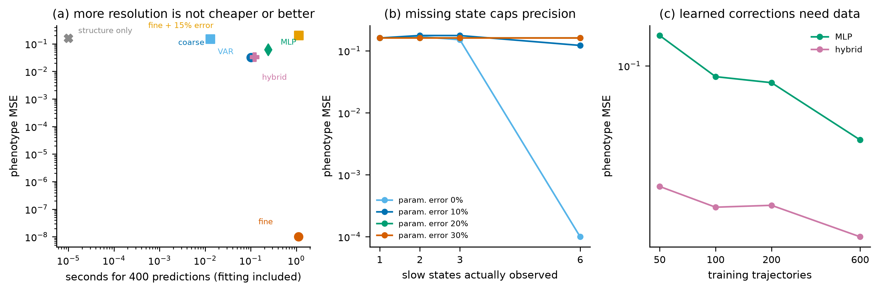
最刺眼的一行是：细模型在参数完全正确时误差低于 10⁻⁴，成本 1.12 秒；同一模型参数错 15% 后误差升到 0.200，比粗模型（0.032，成本 0.101 秒）差六倍。分辨率本身不保证预测能力；分辨率的收益取决于参数是否配得上它。 这是本文最重要的负面结果，也是”多算几个原子”最容易被误解的地方。

The sharpest row: the fine model has an error below 10⁻⁴ with exact parameters at a cost of 1.12 s; with 15% parameter error its error rises to 0.200, six times worse than the coarse model (0.032, 0.101 s). Resolution alone does not guarantee predictive power; its payoff depends on whether the parameters deserve it. This is the most important negative result here, and the easiest thing to misunderstand about “computing a few more atoms”.

第二块结论关于信息从哪来，而且比”测得更多就更好”更微妙。当六个慢变量只观测到一两个时，参数再准也没用：四条误差曲线都停在 0.161 附近，等于表型本身的方差；只有当六个慢变量全部被观测时，参数精度才成为瓶颈，误差从 3.6e-05（参数无误差）升到 0.161（参数错 30%）。观测与精度不是两个可以互相替代的旋钮，而是两道先后必须通过的门：没有状态，精度无处施展；有了状态，精度决定上限。 这与第 3 节的可辨识性结论是同一件事的两种写法。

The second conclusion is about where information comes from, and it is subtler than “more measurement is better”. When only one or two of the six slow variables are observed, parameter accuracy does not help: all four error curves sit near 0.161, the variance of the phenotype itself; only when all six are observed does parameter precision become the bottleneck, with the error rising from 3.6e-05 (no parameter error) to 0.161 (30% error). Observation and precision are not two interchangeable knobs but two gates that must be passed in order: without the state, precision has nowhere to act; with the state, precision sets the ceiling. This is the identifiability result of Section 3 in another language.

比较的公平性需要单独说明，否则这张图会被读成”粗模型更好”。六个模型拿到的输入并不相同：细模型与粗模型拿到的是同一组初始状态与同一套方程；VAR、MLP 与混合模型还额外拿到训练数据；结构模型只拿到网络结构。成本也只计入了”预测 400 个测试样本”的墙钟时间，包含一次性训练，但没有摊薄到多次调用；如果同一模型要预测十万个样本，训练成本会被摊薄，MLP 的相对位置会改善。测试分布是训练分布内的随机初态，没有测试”跨物种”或”跨环境”的外推。在一个更苛刻的测试分布上，纯数据模型的表现会比图中更差，而不是更好——但这需要单独的实验，不能从这张图直接推断。

Fairness of the comparison needs a separate note, or the figure will be read as “coarse is better”. The six models do not receive the same inputs: the fine and coarse models get the same initial states and the same equations; VAR, MLP and the hybrid also get training data; the structure model gets only the network. Cost counts only the wall-clock time to predict 400 test samples, including one-off fitting but not amortised over repeated calls; if the same model were called a hundred thousand times, training would amortise and the MLP’s position would improve. The test distribution is random initial states inside the training distribution, with no cross-species or cross-environment extrapolation. On a harsher test distribution the purely data-driven models would look worse, not better — but that needs its own experiment and cannot be inferred from this figure.

10. 量子在哪里 / Where quantum mechanics enters

有人会说：再往下还有量子。确实。但量子效应进入生命模型的方式，和”细胞是一台量子计算机”是两件不同的事。先看能量账本：300 K 时 \(kT\) = 0.0259 eV（0.60 kcal/mol）。ATP 水解约 0.32 eV，是 12.4 个 \(kT\)；氢键 0.1–0.2 eV；可见光子 2 eV；C–C 键 3.6 eV。热涨落足以驱动构象与磷酸键，但远不足以激发电子。

Someone will say: go one level deeper and there is quantum mechanics. True. But quantum effects enter a model of life in a different way from “the cell is a quantum computer”. Start with the energy ledger: at 300 K, \(kT\) = 0.0259 eV (0.60 kcal/mol). ATP hydrolysis is about 0.32 eV, or 12.4 \(kT\); hydrogen bonds are 0.1–0.2 eV; a visible photon is 2 eV; a C–C bond is 3.6 eV. Thermal fluctuations drive conformations and phosphate bonds but are far too small to excite electrons.

图 16　(a) 细胞的能量账本，从 kT 到电离能。(b) 5 kcal/mol 势垒下的 WKB 透射率，质子与氘核的对比；0.5 Å 处分别为 3.6e-05 与 1.0e-06。(c) 水中分子叠加态的去相干时间估计：0.1 nm 的叠加在 300 K 下约 5.6e-15 秒内消失，4 K 下也只有 3.7e-12 秒。(d) 300 K 下电子激发态的热占据率：2 eV 的能隙对应 2.5e-34。 | Figure 16. (a) The energy ledger of a cell, from kT to ionisation. (b) WKB transmission through a 5 kcal/mol barrier for a proton and a deuteron: 3.6e-05 versus 1.0e-06 at 0.5 Å. (c) Estimated decoherence time of a molecular superposition in water: a 0.1 nm superposition dies in about 5.6e-15 s at 300 K and 3.7e-12 s even at 4 K. (d) Thermal population of an electronic excited state at 300 K: a 2 eV gap corresponds to 2.5e-34.

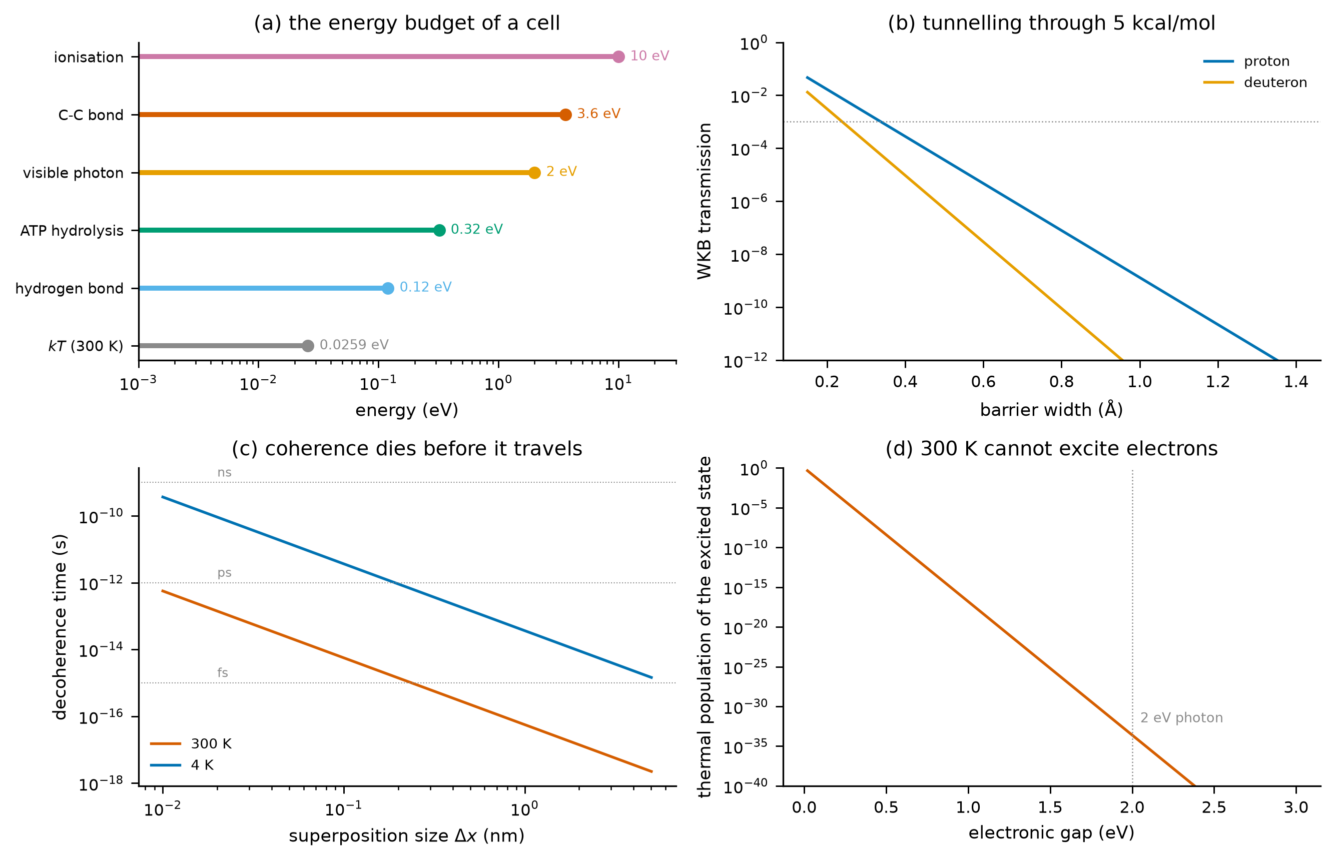
这组数字支持的结论是分层的：量子力学决定规则，但不维持细胞尺度的相干性。 键的断裂与形成、质子与氢负离子的转移、酶催化中的隧穿、光化学与自旋选择，都必须用量子力学；这些效应以能量、速率常数与选择规则的形式进入模型。而一个跨越 0.1 nm 以上的相干叠加，在水的碰撞环境中只能存活飞秒量级，不足以承载细胞尺度的”量子计算”。因此虚拟细胞的正确形态不是”解薛定谔方程到细胞”，而是”用量子化学定参数，用随机动力学描述状态”。

The numbers support a layered conclusion: quantum mechanics sets the rules but does not sustain coherence at cellular scales. Bond breaking, proton and hydride transfer, tunnelling in enzyme catalysis, photochemistry and spin selection all require quantum mechanics; they enter a model as energies, rate constants and selection rules. A coherent superposition spanning more than about 0.1 nm survives only femtoseconds in the collisional environment of water, far too short to carry cell-scale “quantum computation”. The right shape for a virtual cell is therefore not “solve Schrödinger up to the cell” but “fix parameters with quantum chemistry and describe states with stochastic dynamics”.

这里要留一个诚实的缺口：去相干估计用的是一阶碰撞模型，真实体系里存在对称性保护的相干（例如光合复合物中的部分激发态），本文的估计不排除这些特例。它们改变的是参数的来源，不是本节的结构性结论。 量子效应越强，它越像一个需要被测量、被写进速率的边界条件，而不是一个可以免费获得的并行计算资源。

An honest gap remains: the decoherence estimate uses a first-order collisional model, and symmetry-protected coherence does exist in real systems (some excited states in photosynthetic complexes, for example). The estimate here does not rule those cases out. They change where the parameters come from, not the structural conclusion of this section. The stronger a quantum effect is, the more it behaves like a boundary condition that must be measured and written into rates, rather than a parallel-computing resource available for free.

11. 一个可检验的充分性框架 / A testable sufficiency framework

把十组实验放在一起，可以得到一个分层的记账，以及三个互相独立的门槛。

Putting the ten experiments together yields a layered bookkeeping and three independent gates.

图 17　跨尺度记账：每一层的状态变量、时间与空间分辨率，以及约束它的测量方式。层与层之间不是”谁推出谁”，而是”谁的参数由谁提供”。 | Figure 17. Cross-scale bookkeeping: state variables, time and space resolution, and the measurement that constrains each layer. The relation between layers is not “which derives which” but “which supplies whose parameters”.

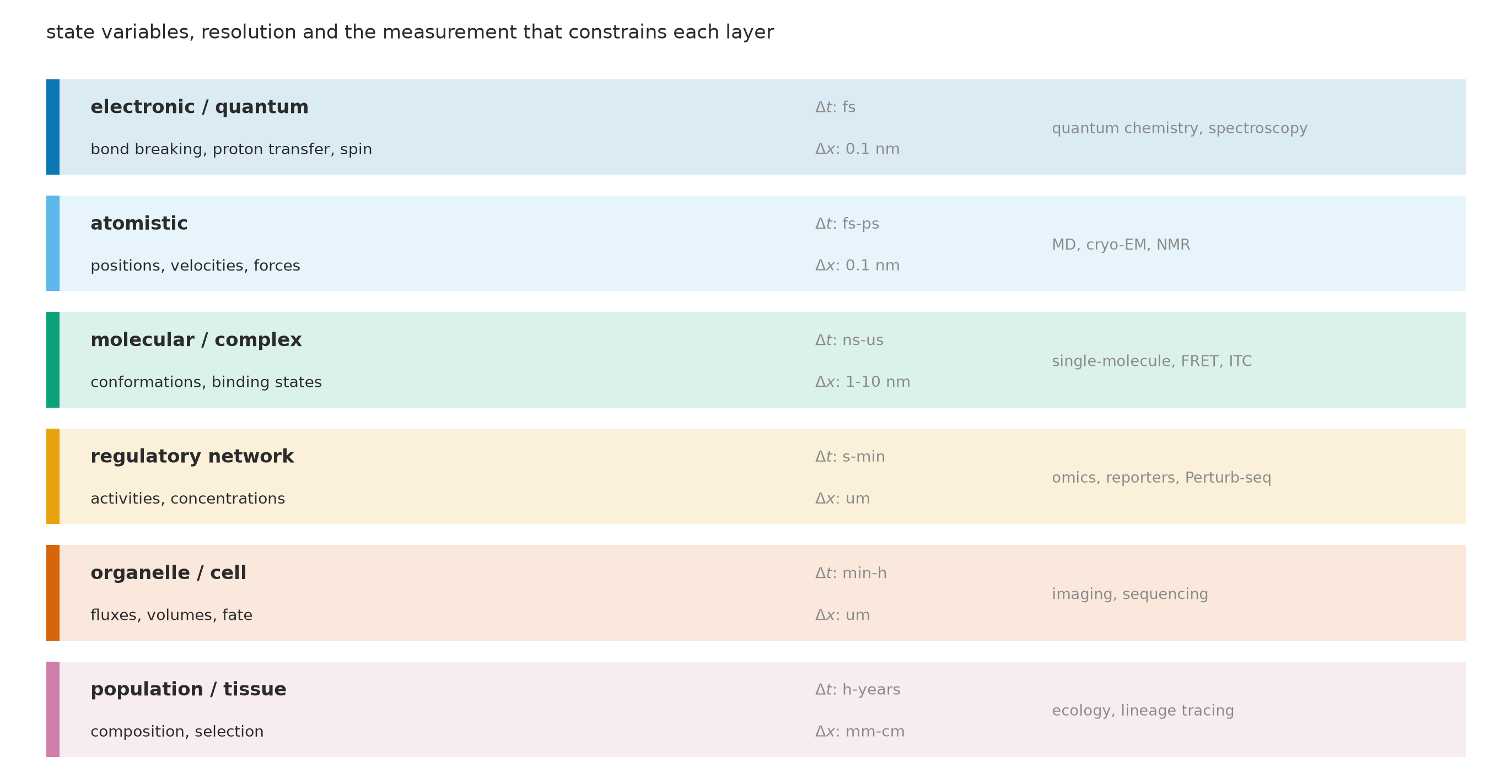
图 17 只画出了三列，但每一层还需要另外五样东西，而且它们比分辨率更难获得：初始条件（每一层都需要上一层的输出作为输入，而上一层往往只给出分布而不是一个点）、动力学方程（在原子层是力场，在网络层是速率方程，在细胞层往往是未知的）、参数及其估计方式（从量子化学、单分子实验或群体拟合，误差结构完全不同）、边界条件（细胞膜、核膜、组织边界，往往决定稳态）、以及误差与不确定性的传播方式（第 7 节的级联放大就是一个例子）。把这五列补齐，比把任何一列的分辨率提高一档都更有价值。

Figure 17 shows three columns, but every layer also needs five more things, and they are harder to obtain than resolution: initial conditions (each layer takes the previous layer’s output as input, and that output is usually a distribution rather than a point), dynamical equations (a force field at the atomic layer, rate equations at the network layer, often unknown at the cell layer), parameters and how they are estimated (quantum chemistry, single-molecule experiments or population fitting have very different error structures), boundary conditions (membrane, nuclear envelope, tissue boundary — often what fixes the steady state), and how error and uncertainty propagate (the cascade amplification of Section 7 is one example). Filling in these five columns is worth more than one more notch of resolution in any single one.

图 18　三个门槛：可辨识性、动力学封闭性、计算可处理性。正确的微观物理不自动保证任何一个；三者都通过，才谈得上”预测充分”。 | Figure 18. Three gates: identifiability, dynamical closure and computational tractability. Correct microphysics does not automatically guarantee any of them; passing all three is what “predictively sufficient” means here.

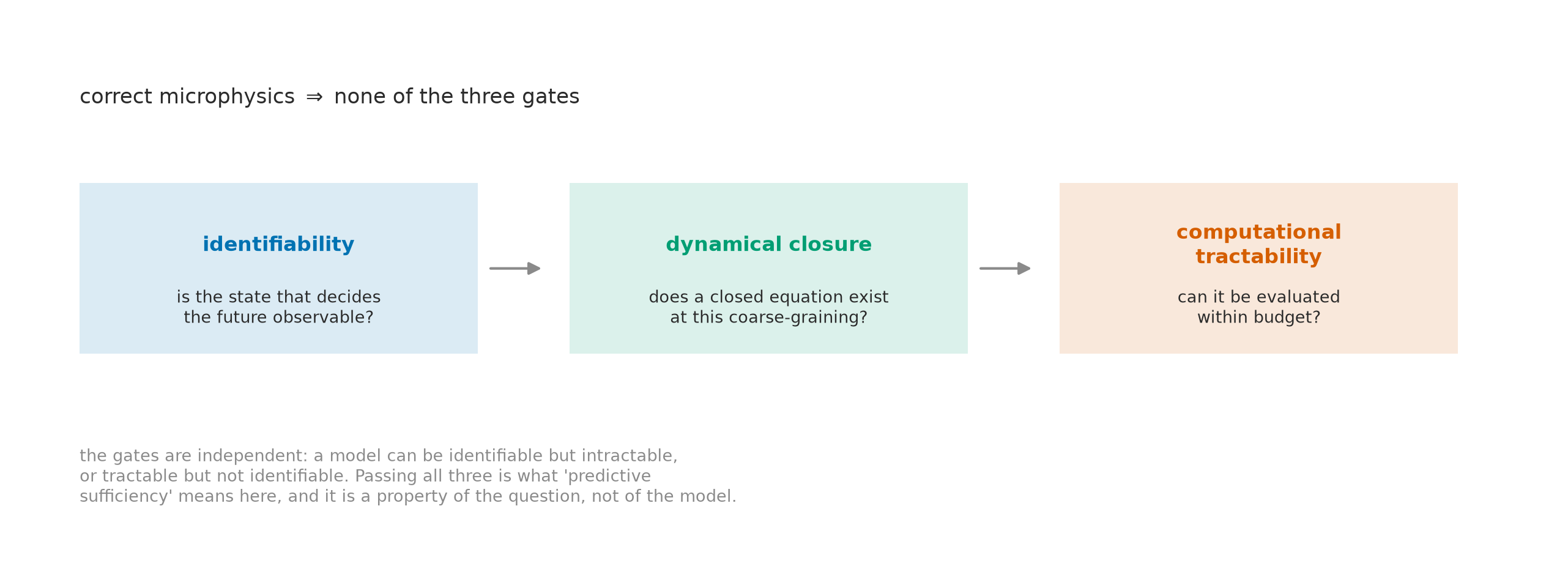
这个框架不是定理，也不假装是定理。它是一张检查表：面对一个”虚拟细胞”的声明，依次问三个问题。（1）决定这个表型的隐藏状态，是否被观测到了？第 3 节的贝叶斯界给出定量版本。（2）在这个粗粒化上，是否存在封闭方程？第 4 节的 ε 给出定量版本。（3）在预算内能否解出？第 2 节与第 9 节给出定量版本。三个问题的答案都是”是”，才可以说这个模型对该问题是预测充分的；否则它只是对一个更窄问题的预测器，这本身没有错，但必须说清楚是哪个更窄的问题。

The framework is not a theorem and does not pretend to be one. It is a checklist: for any claim of a “virtual cell”, ask three questions in order. (1) Is the hidden state that decides this phenotype observed? The Bayes bound of Section 3 gives a quantitative version. (2) Does a closed equation exist at this coarse grain? The ε of Section 4 gives a quantitative version. (3) Can it be solved within budget? Sections 2 and 9 give quantitative versions. Only when all three answers are yes is the model predictively sufficient for that question; otherwise it is a predictor for a narrower question, which is fine, provided the narrower question is named.

12. 回到最初的问题 / Back to the first question

如果生命的所有活动最终都服从物理规律，为什么从物理规律出发并不自动意味着能有效预测生命？本文给出的回答由五个区分组成，而不是一个”生命很复杂”的断言。

If everything a living cell does is ultimately governed by physics, why does starting from physics not automatically let us predict it? The answer offered here consists of five distinctions, not the assertion that “life is complicated”.

可还原性 ≠ 可辨识性。 结构、浓度与观测不足以唯一确定隐藏状态；第 3 节给出了具体的贝叶斯界，而增加观测（RNA、染色质）可以把界降低。可辨识性 ≠ 封闭性。 即使状态已知，粗粒化方程也需要记忆项；第 4 节给出误差随 ε 的定量增长。封闭性 ≠ 可处理性。 一个封闭的方程仍可能算不完；第 2 节给出从原子数到墙钟年数的映射。可处理性 ≠ 预测充分。 一个能在预算内跑完的模型，可能因为参数误差而输给更粗的模型；第 9 节给出了这个反例。

Reducibility ≠ identifiability. Structure, concentrations and observations do not uniquely fix the hidden state; Section 3 gives an explicit Bayes bound, and adding observations (RNA, chromatin) lowers it. Identifiability ≠ closure. Even with the state known, a coarse-grained equation needs memory; Section 4 quantifies how the error grows with ε. Closure ≠ tractability. A closed equation may still be unsolvable; Section 2 maps atom count to wall-clock years. Tractability ≠ sufficiency. A model that runs within budget can lose to a coarser one because of parameter error; Section 9 gives that counterexample.

那么，“理解生命”是否意味着追踪每一个原子？本文的证据说不是。真正需要被保留的，是那些在跨尺度过程中不能被平均掉的信息：决定命运的那个隐藏维度（第 3、6 节）、通量与驱动（第 5 节）、空间结构（第 8 节）、以及参数不确定性的方向（第 7 节）。这些信息有的存在于状态里，有的存在于通量里，有的存在于空间分布里，有的只存在于扰动响应里。找到它们，比把分辨率再提高一档更重要。

So does “understanding life” mean tracking every atom? The evidence here says no. What must be retained is the information that cannot be averaged away across scales: the hidden dimension that decides fate (Sections 3 and 6), fluxes and drive (Section 5), spatial structure (Section 8), and the direction of parameter uncertainty (Section 7). Some of this lives in the state, some in the flux, some in the spatial distribution, some only in perturbation responses. Finding it matters more than one more notch of resolution.

这也是本文对”虚拟细胞”的正面建议：不是一个万能模型，而是一组分工明确的模型——用量子化学与全原子模拟提供参数与机制，用带记忆的粗粒化方程提供可算的动力学，用扰动数据约束因果结构，用空间模型检验混合近似的有效性，用不确定性量化说明预测在什么范围内可信。第 9 节的混合模型以细模型约十分之一的成本达到粗模型的精度，第 3 节的贝叶斯分析说明额外观测的边际价值，这些都是可以立刻执行的设计原则。

This is also the constructive proposal for virtual cells: not one universal model but a division of labour — quantum chemistry and all-atom simulation supply parameters and mechanisms; coarse-grained equations with memory supply computable dynamics; perturbation data constrain causal structure; spatial models test when the well-mixed approximation holds; uncertainty quantification states where a prediction is trustworthy. The hybrid of Section 9 approaches the coarse model at a tenth of the cost, and the Bayes analysis of Section 3 prices additional observations. These are design principles that can be executed now.

如果要把这篇文章变成一个可执行的计划，可以给出三条可以被证伪的预测。第一，带记忆核的粗粒化模型应当在 ε 处于 0.1–1 的细胞过程上系统性地优于无记忆模型，优势随 ε 增大；如果实验发现优势与 ε 无关，本文第 4 节的机制解释就是错的。第二，增加隐藏状态的测量应当比提高同一状态的测量精度更能降低干预预测误差；如果相反，第 3 节的信息论证就需要修补。第三，在 λ/L 接近 1 的系统中，零维模型的干预预测应当出现系统性偏差，而偏差的方向可以由空间模型预测；如果零维模型在这种系统上仍然无偏，第 8 节的结构误差论证就站不住。三条预测都可以在一个设计良好的 Perturb-seq 或微流控实验里被检验，而且都不需要全原子模拟。

To turn this essay into an executable plan, three falsifiable predictions can be stated. First, coarse-grained models with a memory kernel should systematically beat memoryless models on cellular processes with ε between 0.1 and 1, with the advantage growing in ε; if experiment finds no ε-dependence, the mechanism of Section 4 is wrong. Second, adding measurements of hidden states should reduce intervention-prediction error more than increasing the precision of the same measurement; if the opposite holds, the information argument of Section 3 needs repair. Third, in systems with λ/L near one, zero-dimensional models should show a systematic bias in intervention prediction whose sign the spatial model predicts; if the flask stays unbiased there, the structural-error argument of Section 8 does not stand. All three can be tested in a well-designed Perturb-seq or microfluidic experiment, and none requires an all-atom simulation.

最后是本文没有做到的事，必须写清楚。所有”细胞”都是玩具模型，维数与参数远小于真实细胞；成本模型用的是公开基准与理想弱扩展，真实并行效率、I/O 与负载均衡都会让数字更差而不是更好；量子部分用的是量级估计，不构成对具体量子生物学效应的否定；第 9 节的”细模型”是一个十二维 ODE，不是全原子模拟，它证明的是”分辨率与参数误差的权衡”这一逻辑，而不是某个具体的全原子流程的性能。这些限制不改变结论的方向，但改变结论的强度：本文主张的是一种有条件的、可检验的悲观——不是”永远做不到”，而是”在可预见的预算内，正确的做法不是把所有原子都算一遍”。

Finally, what this article did not do must be stated. Every “cell” is a toy model with far fewer dimensions and parameters than a real cell; the cost model uses published benchmarks and ideal weak scaling, and real parallel efficiency, I/O and load balance will make the numbers worse, not better; the quantum section is an order-of-magnitude estimate and does not refute any specific claim of quantum biology; the “fine model” of Section 9 is a twelve-dimensional ODE, not an all-atom simulation, so it establishes the logic of the resolution-versus-parameter-error trade-off rather than the performance of a particular all-atom pipeline. These limits do not change the direction of the conclusion but its strength: what is argued here is a conditional, testable pessimism — not “never”, but “within any foreseeable budget, the right move is not to compute every atom”.

参考文献 / References

1. Schrödinger, E. (1944). What Is Life? Cambridge University Press. (book; no DOI)
2. Turing, A. M. (1952). The chemical basis of morphogenesis. Philosophical Transactions of the Royal Society B 237, 37–72. doi:10.1098/rstb.1952.0012
3. Zwanzig, R. (2001). Nonequilibrium Statistical Mechanics. Oxford University Press. (book; no DOI)
4. Mori, H. (1965). Transport, collective motion, and Brownian motion. Progress of Theoretical Physics 33, 423–455. doi:10.1143/PTP.33.423
5. Gillespie, D. T. (1977). Exact stochastic simulation of coupled chemical reactions. Journal of Physical Chemistry 81, 2340–2361. doi:10.1021/j100540a008
6. Schnakenberg, J. (1976). Network theory of microscopic and macroscopic behavior of master equation systems. Reviews of Modern Physics 48, 571–585. doi:10.1103/RevModPhys.48.571
7. Meinhardt, H., & Gierer, A. (2000). Pattern formation by local self-activation and lateral inhibition. BioEssays 22, 753–760. doi:10.1002/1521-1878(200008)22:8<753::AID-BIES9>3.0.CO;2-Z
8. Thornburg, Z. R., et al. (2022). Fundamental behaviors emerge from simulations of a living minimal cell. Cell 185, 345–360. doi:10.1016/j.cell.2021.12.025
9. Stevens, J. A., et al. (2023). Molecular dynamics simulation of an entire cell. Frontiers in Chemistry 11, 1106495. doi:10.3389/fchem.2023.1106495
10. Shaw, D. E., et al. (2021). Anton 3: twenty microseconds of molecular dynamics simulation before lunch. SC21. doi:10.1145/3458817.3487397
11. Abraham, M. J., et al. (2015). GROMACS: high performance molecular simulations through multi-level parallelism. SoftwareX 1–2, 19–25. doi:10.1016/j.softx.2015.06.001
12. Vanommeslaeghe, K., et al. (2010). CHARMM general force field. Journal of Computational Chemistry 31, 671–690. doi:10.1002/jcc.21367
13. Marrink, S. J., et al. (2023). The Martini model in materials science. Chemical Reviews 123, 10505–10553. doi:10.1021/acs.chemrev.2c00778
14. Unke, O. T., et al. (2021). Machine learning force fields. Chemical Reviews 121, 10142–10186. doi:10.1021/acs.chemrev.0c01111
15. Bussi, G., & Parrinello, M. (2007). Accurate sampling using Langevin dynamics. Physical Review E 75, 056707. doi:10.1103/PhysRevE.75.056707
16. Elowitz, M. B., Levine, A. J., Siggia, E. D., & Swain, P. S. (2002). Stochastic gene expression in a single cell. Science 297, 1183–1186. doi:10.1126/science.1070919
17. Ferrell, J. E., & Machleder, E. M. (1998). The biochemical basis of an all-or-none cell fate switch. Science 280, 895–898. doi:10.1126/science.280.5365.895
18. Kholodenko, B. N. (2006). Cell-signalling dynamics in time and space. Nature Reviews Molecular Cell Biology 7, 165–176. doi:10.1038/nrm1838
19. Rao, C. V., & Arkin, A. P. (2003). Stochastic chemical kinetics and the quasi-steady-state assumption. Journal of Chemical Physics 118, 4999–5010. doi:10.1063/1.1543588
20. Lambert, N., et al. (2013). Quantum biology. Nature Physics 9, 10–18. doi:10.1038/nphys2474
21. Klinman, J. P., & Kohen, A. (2013). Hydrogen tunnelling links protein dynamics to enzyme catalysis. Annual Review of Biochemistry 82, 471–496. doi:10.1146/annurev-biochem-051710-133623
22. Zurek, W. H. (2003). Decoherence, einselection, and the quantum origins of the classical. Reviews of Modern Physics 75, 715–775. doi:10.1103/RevModPhys.75.715
23. Bunne, C., et al. (2023). Learning single-cell perturbation responses using neural optimal transport. Nature Methods 20, 1759–1768. doi:10.1038/s41592-023-01969-x

说明：第 1–3 条为经典著作，第 4–22 条给出 DOI，第 23 条为单细胞扰动建模的近期工作。成本模型的两个基准分别来自第 10 与第 11 条的公开性能数据；所有算法细节与常数在 experiments/README.md 中列出。

Note: entries 1–3 are classic books; 4–22 carry DOIs; 23 is recent work on single-cell perturbation modelling. The two cost benchmarks come from the published performance numbers in entries 10 and 11; all algorithmic details and constants are listed in experiments/README.md.