本文由 AI(DeepSeek-Flash) 检索、整理并撰写,尚未经过人工逐条校对。文中所有数字、曲线与图像都由随文 R 代码现场计算生成,随机过程统一设定了种子,因此结果可复现;模拟里用到的参数是教学用的简化值,不应当作真实物种的定量结论。生命起源与进化生物学中仍有大量争议,凡涉及争议处,文中会直接说明”这是模型假设”而不是”这是事实”。
This article was researched and written by an AI system (DeepSeek-Flash) and has not been proofread line by line by a human. Every number, curve and figure is computed by the R code in this post with fixed seeds, so the results reproduce; the parameter values in the simulations are teaching simplifications, not quantitative claims about real species. Several questions in origin-of-life research and evolutionary biology remain contested, and wherever that is the case the text says “this is a model assumption” rather than “this is a fact”.
生成本文所用的提示词(压缩后) / Prompt used to generate this article (condensed)
写一篇长文中英对照文章,题目《进化是一种搜索算法吗?生命如何探索近乎无限的可能性》,关键词 Fitness Landscape · Evolutionary Search · Optimization。围绕五个问题展开:搜索空间的规模、适应度景观与局部最优、选择–漂变–突变偏向的相对作用、可进化性、开放式进化。要求:数学定义写清楚(Price 方程、replicator 方程、Wright–Fisher 固定概率、Eigen 错误阈值、NK 模型),所有图用 R 现场生成(3D 景观、NK 模型、进化轨迹、系统发育树、基因型网络、中性网络、种群动态),能放进一个统一框架就把自然选择、贝叶斯推断、梯度下降、强化学习和开放式进化放在同一组更新方程下比较;最后一节讨论数字进化与可进化 AI 的最新争论。禁止编造文献 DOI。
Write a long bilingual post, “Is Evolution a Search Algorithm? How Life Explores Nearly Infinite Possibilities”, keywords Fitness Landscape · Evolutionary Search · Optimization. Cover five questions: the size of genotype space, fitness landscapes and local optima, the relative roles of selection, drift and mutation bias, evolvability, and open-endedness. Make the mathematics explicit (Price equation, replicator equation, Wright–Fisher fixation probability, Eigen’s error threshold, the NK model) and generate every figure live in R (3D landscapes, NK models, evolutionary trajectories, phylogenies, genotype networks, neutral networks, population dynamics). If a unified framework is possible, compare natural selection, Bayesian inference, gradient descent, reinforcement learning and open-ended evolution under one family of update rules. End with the current debate on digital evolution and evolvable AI. Do not invent DOIs.
1. 把进化写成一道搜索题 / Writing evolution as a search problem
先做一个思想实验。假设你是一个从未见过地球生命的外星工程师,有人递给你一份 4.6 Mb 的大肠杆菌基因组,告诉你:这串字符是在四十亿年里、由一堆没有大脑的化学反应”找”出来的,而且它能在 37 °C 的肉汤里自我复制。你大概会问两个问题:它是怎么找到这串字符的?以及,它为什么没有找到更好的?
To start, run a thought experiment. You are an alien engineer who has never seen life on Earth, and someone hands you a 4.6 Mb E. coli genome: this string was “found” over four billion years by a pile of brainless chemistry, and it can copy itself in broth at 37 °C. You would probably ask two questions: how did it find that string, and why did it not find something better?
Every search problem can be written as a triple \((\mathcal{X}, f, \mathcal{A})\): a search space \(\mathcal{X}\) (the set of candidate solutions), an objective \(f: \mathcal{X} \to \mathbb{R}\), and an algorithm \(\mathcal{A}\) that decides where to look next. In gradient descent, \(\mathcal{X} = \mathbb{R}^d\), \(f\) is smooth and differentiable, and \(\mathcal{A}\) uses \(\nabla f\) to pick a direction. In evolution, \(\mathcal{X}\) is the set of all possible genomes, \(f\) is fitness, and \(\mathcal{A}\) is the whole machinery of mutation, inheritance, selection and drift.
Once the analogy is written down, several oddities of evolution become visible immediately. First, it has no gradient: an organism cannot differentiate fitness, it can only be born, survive or die, sampling \(f\) with its life. Second, it searches many points at once: a population is not a point but thousands of points probing in parallel. Third, the objective is not fixed: predators, parasites, climate and conspecifics all move, so \(f\) changes in time, and organisms modify their environment and thereby change \(f\) itself — niche construction.
So the route of this long post is: take the three components apart one at a time (chapters 2–3 for the space and the landscape, chapters 4–6 for the stochastic and structural parts of the algorithm), then discuss evolution’s “meta-abilities” (evolvability and open-endedness in chapters 7–8), and finally reassemble the parts into one mathematical framework and compare it term by term with gradient descent, Bayesian inference and reinforcement learning (chapter 9). By the end you should be able to decide for yourself whether evolution is a search algorithm, and if so, where exactly it differs from the ones we already know.
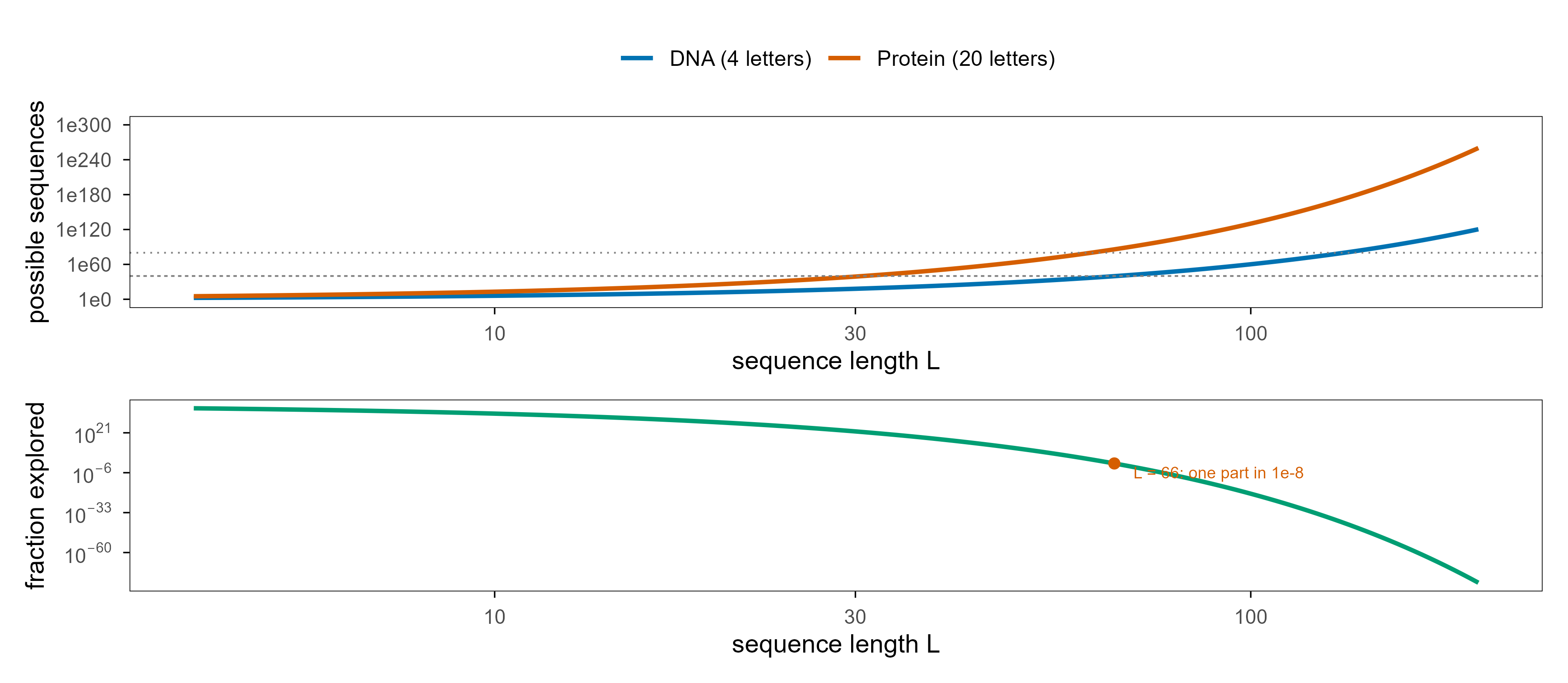
Start with arithmetic. A DNA sequence of length \(L\) has \(4^L\) possible variants; a mere 20-mer already has \(4^{20} \approx 1.1 \times 10^{12}\) variants, a 100-bp coding region has \(4^{100} \approx 1.6 \times 10^{60}\), and a 100-amino-acid protein has \(20^{100} \approx 10^{130}\). For comparison, the observable universe contains about \(10^{80}\) atoms.
Code
len_grid <-exp(seq(log(4), log(200), length.out =160))space_df <-bind_rows(tibble(len = len_grid, alphabet ="DNA (4 letters)", n =4^len_grid),tibble(len = len_grid, alphabet ="Protein (20 letters)", n =20^len_grid))p_space_a <-ggplot(space_df, aes(len, n, colour = alphabet)) +geom_line(linewidth =0.9) +geom_hline(yintercept =c(10^40, 10^80), linetype =c("22", "13"),colour = blog_pal[["grey"]], linewidth =0.35) +scale_colour_manual(values =unname(blog_pal[c("blue", "vermillion")])) +scale_x_log10() +scale_y_log10(breaks =10^seq(0, 300, by =60),labels =function(x) paste0("1e", round(log10(x))),limits =c(1, 1e300)) +labs(x ="sequence length L", y ="possible sequences", colour =NULL) +theme(legend.position ="top")explored <-tibble(len = len_grid, fraction =10^40/4^len_grid)p_space_b <-ggplot(explored, aes(len, fraction)) +geom_line(linewidth =0.9, colour = blog_pal[["green"]]) +scale_x_log10() +scale_y_log10(label =label_log()) +annotate("point", x =66, y =10^40/4^66, colour = blog_pal[["vermillion"]], size =1.8) +annotate("text", x =70, y =10^(-6), label ="L = 66: one part in 1e-8",size =2.5, hjust =0, colour = blog_pal[["vermillion"]]) +labs(x ="sequence length L", y ="fraction explored")p_space_a / p_space_b
Figure 1: 搜索空间的量级。左:DNA(4 字母)与蛋白质(20 字母)序列空间随长度指数增长;两条水平线分别是可观测宇宙的原子数(约 10^80)与生物圈有史以来尝试过的突变总量(粗略量级 10^40)。右:已被探索的比例随长度迅速跌破任何可想象的阈值。 | The scale of the search space. Left: sequence space grows exponentially with length for DNA (4 letters) and proteins (20 letters); the two horizontal lines mark the number of atoms in the observable universe (about 10^80) and a rough order-of-magnitude estimate of every mutation the biosphere has ever tried (10^40). Right: the fraction explored falls below any imaginable threshold as length grows.
It is worth staring at the right-hand curve for a few seconds. Even counting every replication and every mutation the biosphere has performed in four billion years, the fraction of sequence space explored beyond length 66 is already below \(10^{-8}\); for a protein the fraction is too small to write a meaningful exponent. Life is not enumerating. It is sampling extremely sparsely in a space that is almost entirely empty.
This sets the tone for everything that follows. Since enumeration is impossible, “finding a good solution” can only rely on two things: whether the search algorithm concentrates its samples in promising regions, and whether the structure of the space allows locally useful changes to accumulate. The first is a question about algorithms, the second about landscapes. They are two sides of one coin — a fitness landscape is just the shape you get by laying the values of \(f\) over the space.
3. 适应度景观:进化是在爬山吗 / Fitness landscapes: is evolution hill climbing?
The idea of a fitness landscape was introduced by Sewall Wright in 1932 as a metaphor: lay genotypes on a plane, plot fitness as height, and evolution becomes a path across the landscape. The metaphor is extremely successful and extremely dangerous, because it suggests that the landscape is fixed, two-dimensional and graspable by eye. In reality the dimension equals the number of genes, the landscape changes with the environment, and organisms reshape the terrain themselves.
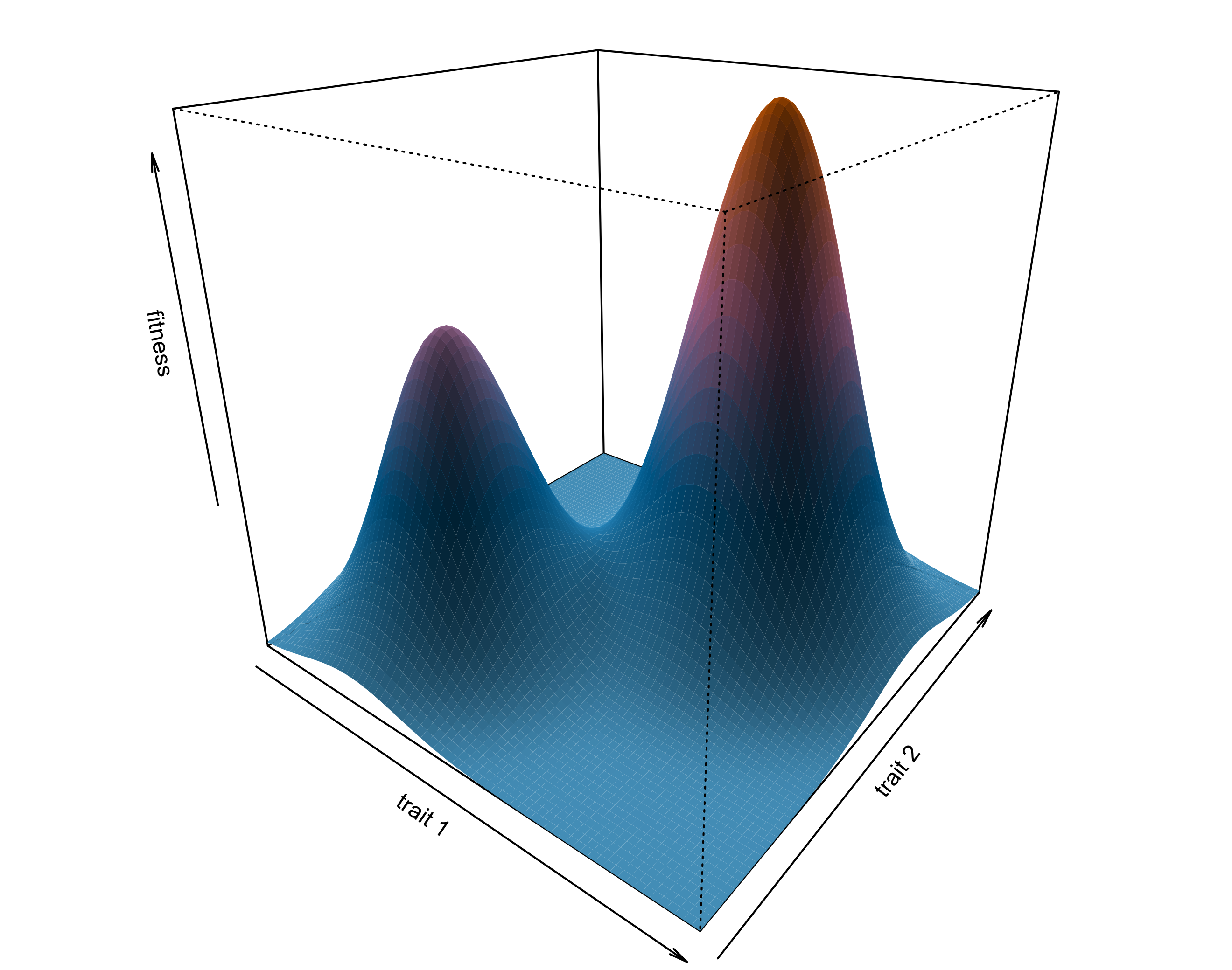
尽管有这些限制,二维景观仍然是理解”为什么会卡住”的最好玩具。考虑下面这个有两个峰的地形:
Despite these caveats, a two-dimensional landscape is still the best toy for understanding why search gets stuck. Consider the two-peaked terrain below:
Figure 2: 一个教学用的适应度景观:两个高度不同的峰,外加一个很小的肩部。真实景观的维度等于基因数,这里压到二维只为了能画出来。 | A teaching landscape: two peaks of unequal height plus a small shoulder. A real landscape has as many dimensions as genes; it is squashed to two here only so that it can be drawn.
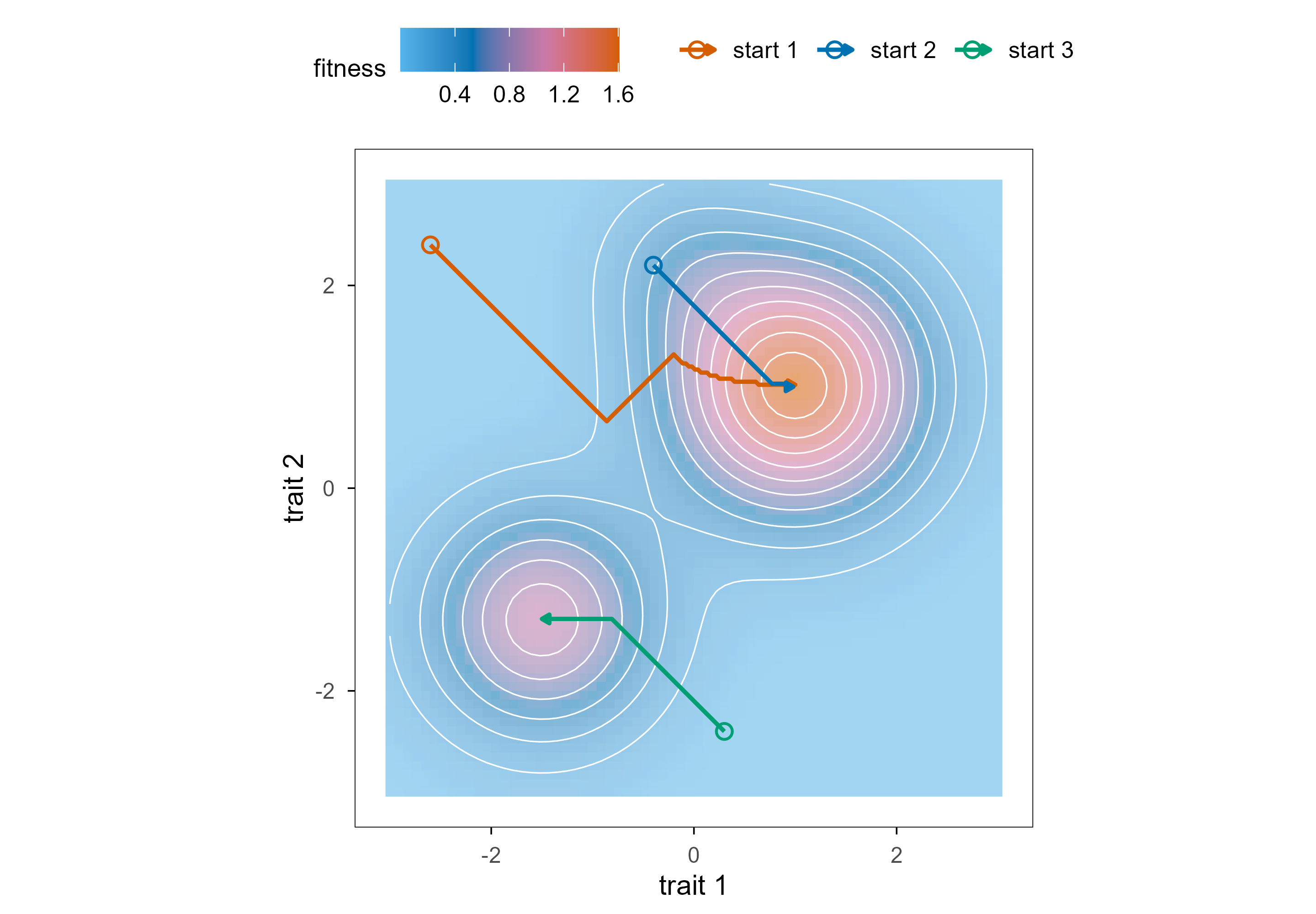
If you drop a population on this terrain and let it do one thing only — move to a higher neighbour whenever one exists — which peak does it reach? The answer depends on where it starts. The figure below draws three such hill-climbing paths whose starting points differ only slightly but whose endpoints are two completely different peaks.
Figure 3: 同一景观上的三条爬山轨迹。起点只差 0.2 个坐标单位,两条落在较高的峰,一条落在较低的峰——这就是路径依赖(path dependence)。灰线是等高线,等高线越密说明坡越陡。 | Three hill-climbing paths on the same landscape. The starting points differ by 0.2 units, yet two paths end on the higher peak and one on the lower peak: path dependence. Grey lines are contours; denser contours mean steeper slopes.
This is what “local optimum” means: a point whose every neighbour is worse, yet which is not the global best. For gradient descent this is fatal — a first-order method has no mechanism for knowing that a taller mountain lies beyond. Evolution also gets stuck, but the real question is whether it can escape, and that depends on population size, ruggedness and the other sources of randomness available.
要让”崎岖”从形容词变成可计算的量,最常用的工具是 Stuart Kauffman 在 1989 年提出的 NK 模型。规则很简单:\(N\) 个基因座,每个基因座对适应度的贡献取决于它自己和另外 \(K\) 个基因座,总适应度是 \(N\) 个贡献的平均:
To turn “rugged” from an adjective into a computable quantity, the standard tool is the NK model of Stuart Kauffman (1989). The rule is simple: there are \(N\) loci, and the contribution of each locus depends on itself plus \(K\) other loci; total fitness is the mean of the \(N\) contributions:
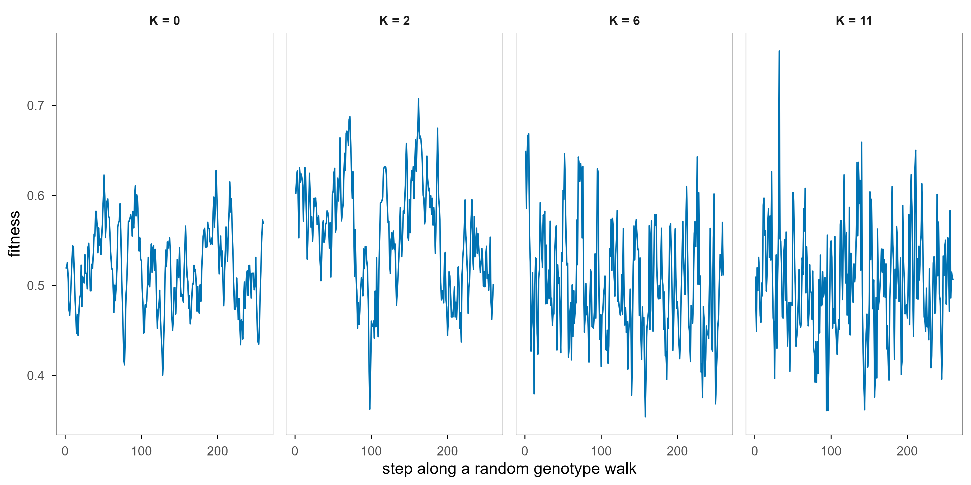
When \(K = 0\) each locus contributes independently, so the landscape is smooth and single-peaked; when \(K = N-1\) every locus interacts with every other, the landscape is fully randomized and studded with local optima. Moving \(K\) from 0 to \(N-1\) is a continuous road from predictable to unpredictable.
Code
nk_slice <-function(N, K, steps =260, seed =1) {set.seed(seed) model <-make_nk(N, K, seed) g <-sample(c(0, 1), N, replace =TRUE) out <-numeric(steps) out[1] <-nk_fit(model, matrix(g, nrow =1))for (s in2:steps) { i <-sample.int(N, 1) g[i] <-1- g[i] out[s] <-nk_fit(model, matrix(g, nrow =1)) }tibble(step =seq_len(steps), fitness = out, K =paste0("K = ", K))}slices <-lapply(c(0, 2, 6, 11), function(k) nk_slice(20, k, seed =7)) |>bind_rows() |>mutate(K =factor(K, levels =paste0("K = ", c(0, 2, 6, 11))))ggplot(slices, aes(step, fitness)) +geom_line(linewidth =0.45, colour = blog_pal[["blue"]]) +facet_wrap(~ K, nrow =1) +labs(x ="step along a random genotype walk", y ="fitness")
Figure 4: NK 模型的崎岖程度随 K 增长。四张图都是沿同一条随机游走路径(每次翻转一个基因座)采样的适应度剖面,N = 20。K = 0 时单步最多只能改变 1/20,剖面是一条被夹在窄带里的细碎行走;K = 11 时单步就能让适应度跳变 0.2 以上,剖面已经没有任何可读结构。 | Ruggedness grows with K in the NK model. Each panel samples fitness along one random walk through genotype space (one locus flipped per step) with N = 20. At K = 0 a single step can change fitness by at most 1/20, so the profile is a fine walk inside a narrow band; at K = 11 one step can move fitness by more than 0.2 and no readable structure remains.
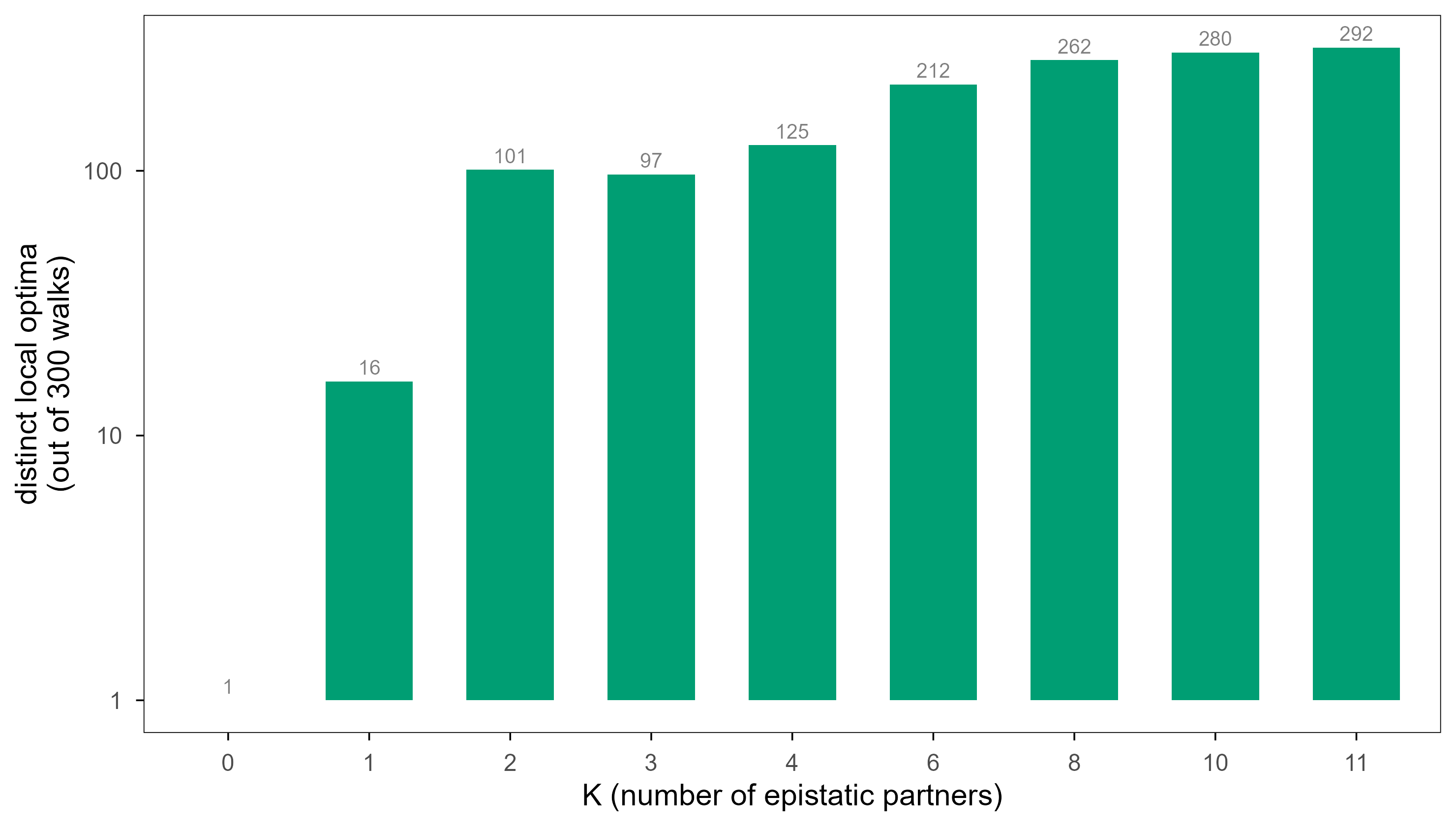
Figure 5: 局部最优的数目随 K 爆炸。每个 K 值从 300 个随机起点各爬一次山,统计落点中互不相同的局部最优数(N = 20,300 次重复的箱线)。K = 0 时全空间只有一个最优,K = 11 时数百个起点落在几十个不同的峰上。 | The number of local optima explodes with K. For each K, 300 random starts climb to a local optimum and distinct endpoints are counted (N = 20; boxes over 300 replicates). At K = 0 the whole space has one optimum; at K = 11 hundreds of starts land on dozens of different peaks.
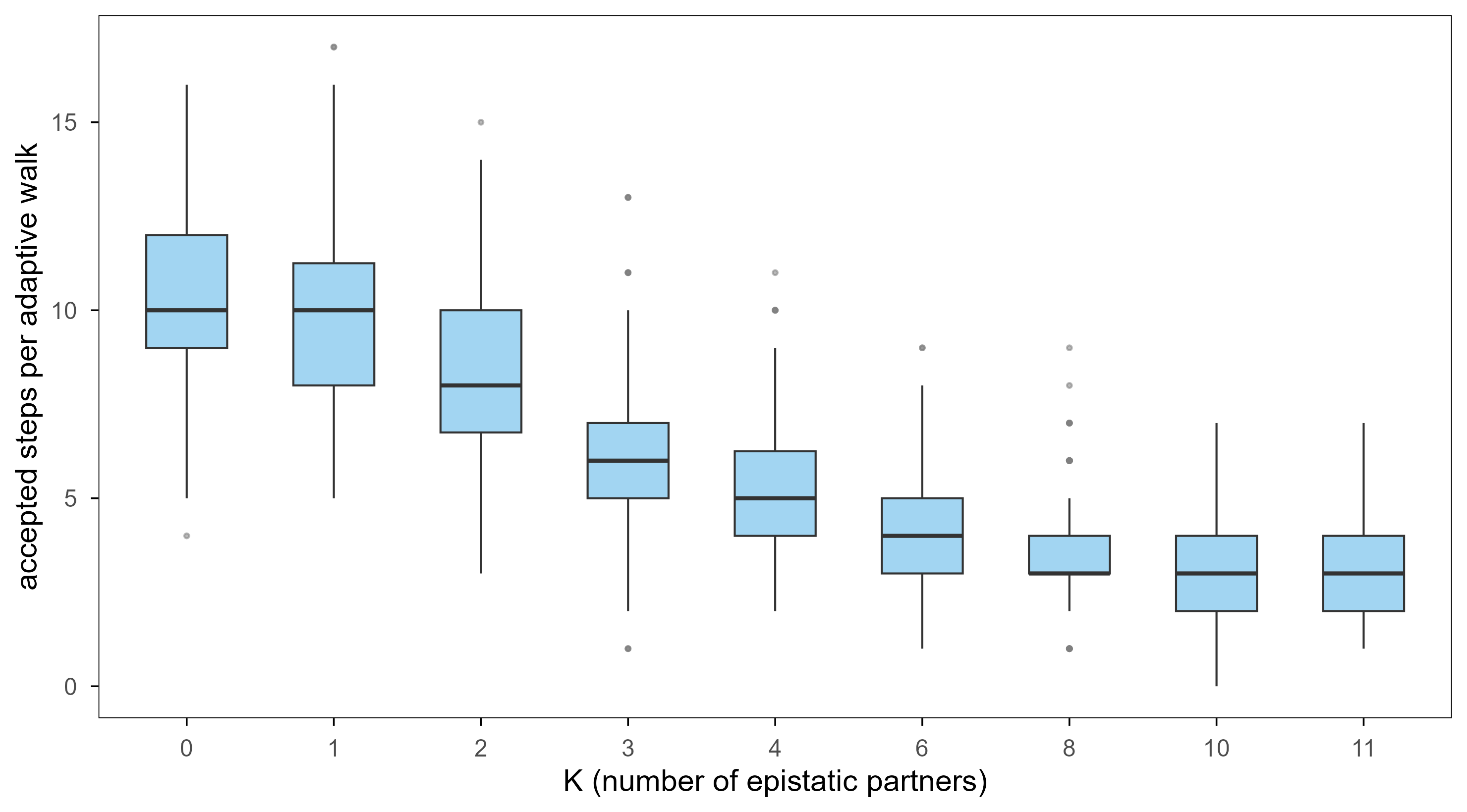
Figure 6: 爬山能走多远也随 K 变化。K 越大,单步改进的空间越小,轮次越短,而且一开始的适应度更低——在崎岖景观上,进化更容易被「锁死」在小台阶上。 | How far hill climbing gets also depends on K. Larger K means fewer improving steps, shorter walks and lower starting fitness: on rugged landscapes evolution is easily locked onto small ledges.
These figures give an uncomfortable conclusion: on rugged landscapes the efficiency of hill climbing drops quickly with \(K\), and the endpoints become increasingly arbitrary. Kauffman used the model to argue that complex organisms remain “evolvable” partly because they keep \(K\) within a workable range — through modularity, redundancy and robustness, turning one spiky landscape into several smooth small ones. That idea returns in chapter 7.
The popular picture of evolution is “natural selection makes organisms better and better”. That sentence is not wrong, but it leaves out two equally important forces: genetic drift and mutation bias. Separating the three is a key step towards answering whether evolution is an optimization algorithm.
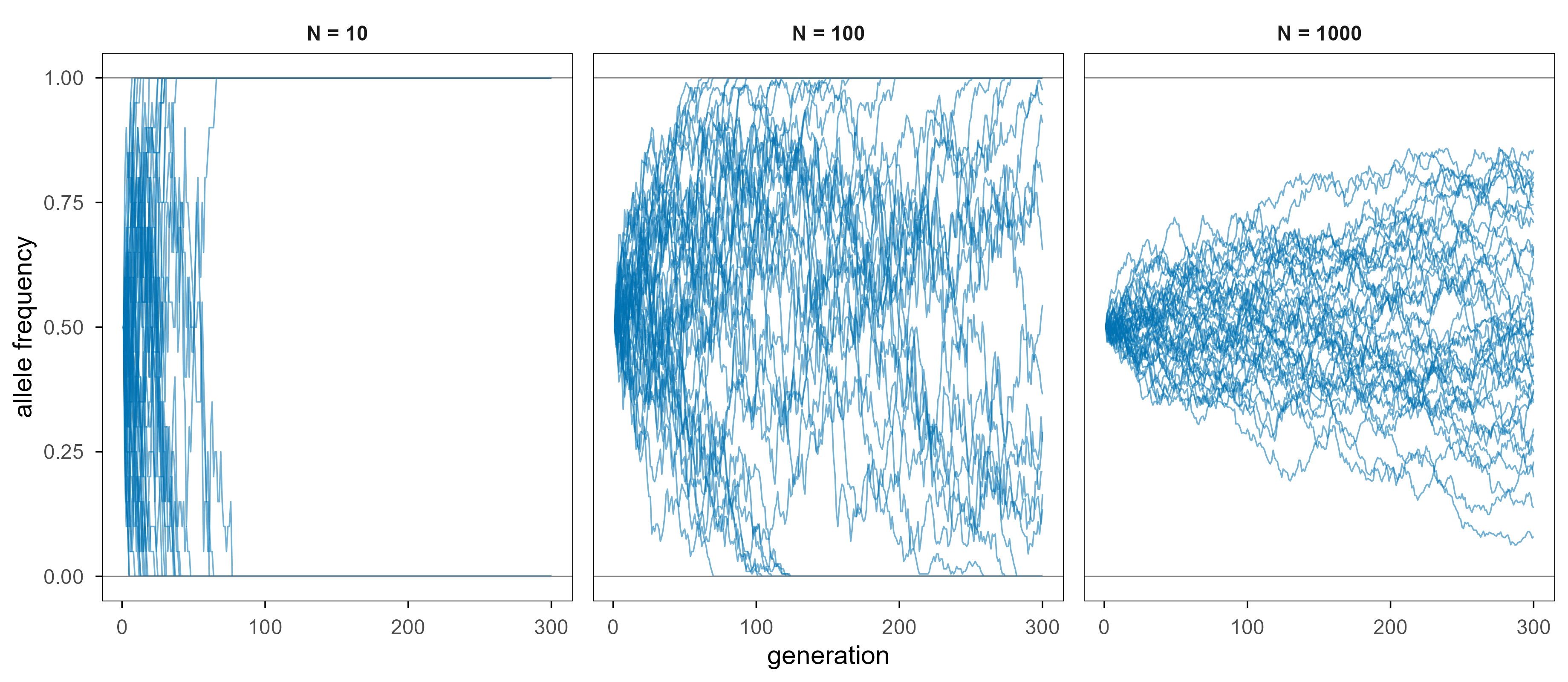
Drift is the inevitable consequence of sampling. Even if every individual has identical fitness, allele frequencies in the next generation are not exactly those of this generation, because reproduction is a finite sample. The smaller the population, the larger the sampling noise. The simulation below draws the purely neutral case (\(s = 0\)); the only thing that differs between the three panels is population size.
Figure 7: 中性漂变。群体越小,等位基因频率的随机游走越快,固定(频率到 0 或 1)越早发生。N = 10 时几十代就固定,N = 1000 时几百代仍在中间徘徊。 | Neutral drift. Smaller populations wander faster and fix (hit frequency 0 or 1) sooner. At N = 10 fixation takes a few dozen generations; at N = 1000 the frequency is still hovering near the middle after hundreds.
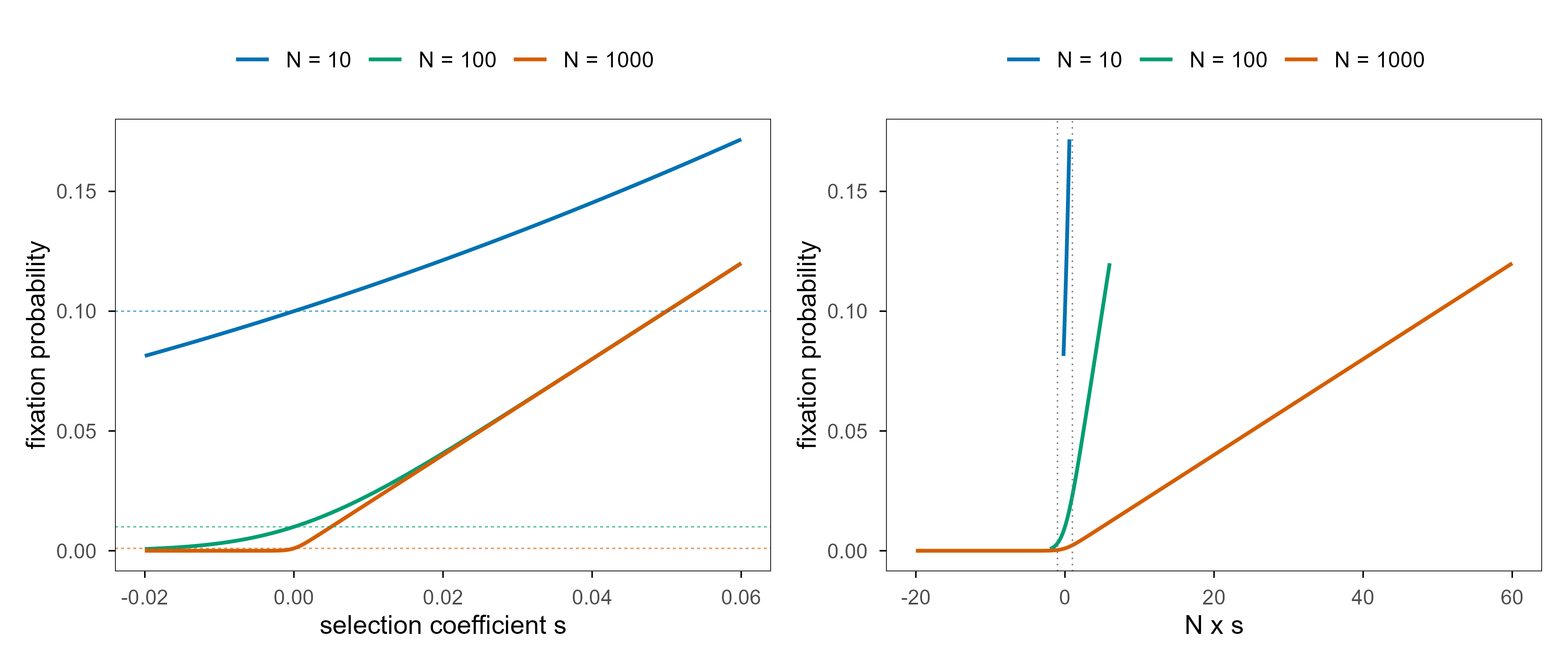
Selection, by contrast, has direction. Kimura’s 1962 diffusion approximation gives a neat result: a new mutation starting at frequency \(1/(2N)\) with a constant selection coefficient \(s\) fixes with probability, for \(|s| \ll 1\),
whose exact form is \((1-e^{-2s})/(1-e^{-2Ns})\), and the two agree for \(|s| \ll 1\). As \(s \to 0\) it reduces to \(1/N\), the neutral expectation under pure drift. The most useful feature of this formula is that it compresses the relative strength of selection and drift into one dimensionless number, \(Ns\): when \(|Ns| \ll 1\) the mutation is effectively neutral, when \(Ns \gg 1\) selection dominates.
Figure 8: 左:固定概率随选择系数变化,三条线的群体大小不同(虚线是中性预期 1/N)。右:把横轴换成 N·s 之后,三条曲线几乎重合——决定命运的不是 s 本身,而是 s 与群体大小的乘积。 | Left: fixation probability against the selection coefficient for three population sizes (dashed line is the neutral expectation 1/N). Right: with N·s on the horizontal axis the three curves nearly collapse — fate is decided by the product of s and population size, not by s alone.
Remember the right-hand panel: \(|Ns| \approx 1\) is a boundary — drift rules to its left, selection to its right. The enormous range of effective population sizes in nature (six orders of magnitude and more) means the same mutation can be invisible noise in one species and a decisive advantage in another.
Mutation bias is the third force: mutations are not uniform across sites — transitions, CpG deamination and slippage in tandem repeats each have their own preferences. Where selection is weak (\(|Ns|\) small) the bias can set the direction of evolution outright; where selection is strong it only biases the proposal distribution.
The most elegant way to put all three into one equation is the Price equation. For any trait \(z\), the change in the mean across one generation decomposes as
The first term is selection — the covariance between trait and fitness; the second is transmission — changes of the trait within individuals during reproduction (mutation, recombination, environment-induced change). Drift is not in this formula because Price’s equation describes an expectation; to include it one replaces the covariance with a finite-sample estimate, and the covariance then acquires a sampling-error term. The detail matters: drift is not a force, it is the error of a finite-sample estimate of selection.
Back to the question from chapter 3: with several peaks, how does evolution get from one to another? Three mechanisms are known, and all are mathematically clear.
The first is drift. Shrink the population until \(|Ns| \lesssim 1\); then downhill and uphill steps are dynamically indistinguishable, and the population can wander across a valley like a drunkard. The price is that it also wanders the wrong way, so drift cuts both ways.
Code
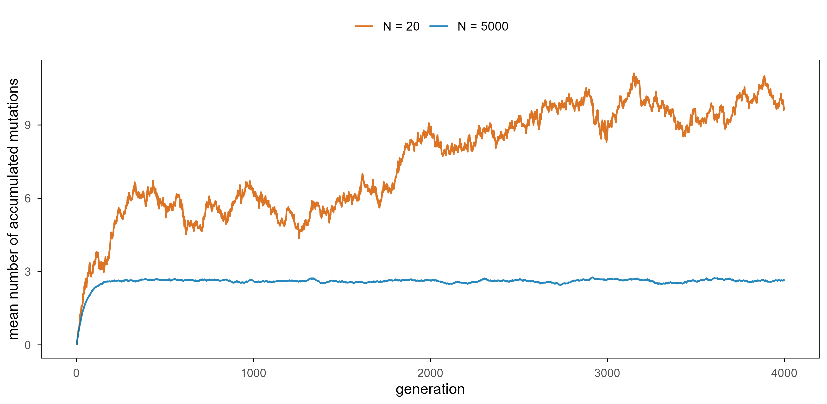
L_val <-20w_val <-0.90+0.10*cos(2* pi * (0:L_val) / L_val)mu_val <-0.05up_val <- mu_val * (L_val - (0:L_val)) / L_valdown_val <- mu_val * (0:L_val) / L_valsim_chain <-function(N, w, up, down, gens, init =1, seed =5) {set.seed(seed) L <-length(w) -1 M <-matrix(0, L +1, L +1)for (k in0:L) { stay <-1- up[k +1] - down[k +1] M[k +1, k +1] <-max(stay, 0)if (k < L) M[k +1, k +2] <- up[k +1]if (k >0) M[k +1, k] <- down[k +1] } n <-numeric(L +1); n[init] <- N mk <- mf <-numeric(gens)for (t inseq_len(gens)) { mk[t] <-sum(n * (0:L)) / N mf[t] <-sum(n * w) / N p <- n * w /sum(n * w) q <-as.vector(p %*% M) q <-pmax(q, 0); q <- q /sum(q) n <-as.vector(rmultinom(1, N, q)) }tibble(gen =seq_len(gens), mean_k = mk, mean_fitness = mf)}valley <-bind_rows(lapply(c(20, 5000), function(n) {bind_rows(lapply(1:6, function(r) sim_chain(n, w_val, up_val, down_val, 4000, seed = r))) |>group_by(gen) |>summarise(mean_k =mean(mean_k), mean_fitness =mean(mean_fitness),.groups ="drop") |>mutate(N =paste0("N = ", n)) }))ggplot(valley, aes(gen, mean_k, colour = N)) +geom_line(linewidth =0.6, alpha =0.85) +scale_colour_manual(values =unname(blog_pal[c("vermillion", "blue")])) +labs(x ="generation", y ="mean number of accumulated mutations", colour =NULL)
Figure 9: 小群体可以穿过适应度低谷,大群体不能。地形是 0 到 20 个突变步上的双峰景观(两端适应度 1.0,中点 0.9,每步选择系数约 0.015)。N = 20 时种群在两峰之间来回游荡,平均累计突变数长到 9 附近;N = 5000 时被钉在出发峰脚下,只带着一点突变负荷(约 2.6)——它拿不到对面那个同样高的峰。 | Small populations cross fitness valleys, large ones cannot. The terrain is a two-peaked landscape over 0–20 mutational steps (fitness 1.0 at both ends, 0.9 in the middle, about 0.015 of selection per step). At N = 20 the population wanders between the two peaks, with the mean number of accumulated mutations rising to about 9; at N = 5000 it stays at the foot of the starting peak with a small mutation load (about 2.6) and never reaches the equally high peak on the other side.
第二种是中性路径。 如果从峰 A 到峰 B 之间存在一条所有点适应度都不下降的路径,那么这条路径在最优化意义上就是”平的”,选择不会阻止种群沿它前进。这类路径是否存在,完全取决于基因型—表型映射的结构,第 6 章会专门处理。
The second is a neutral path. If there is a route from peak A to peak B along which fitness never decreases, that route is flat in the optimisation sense and selection will not block movement along it. Whether such routes exist depends entirely on the structure of the genotype–phenotype map, which is the subject of chapter 6.
The third is recombination. Sex combines favourable mutations carried by two different individuals, which is mathematically a multi-point jump operator in the search. It lets a population bypass intermediate valleys, but it also breaks up favourable combinations (recombination load), and stitching together two distant solutions often produces garbage.
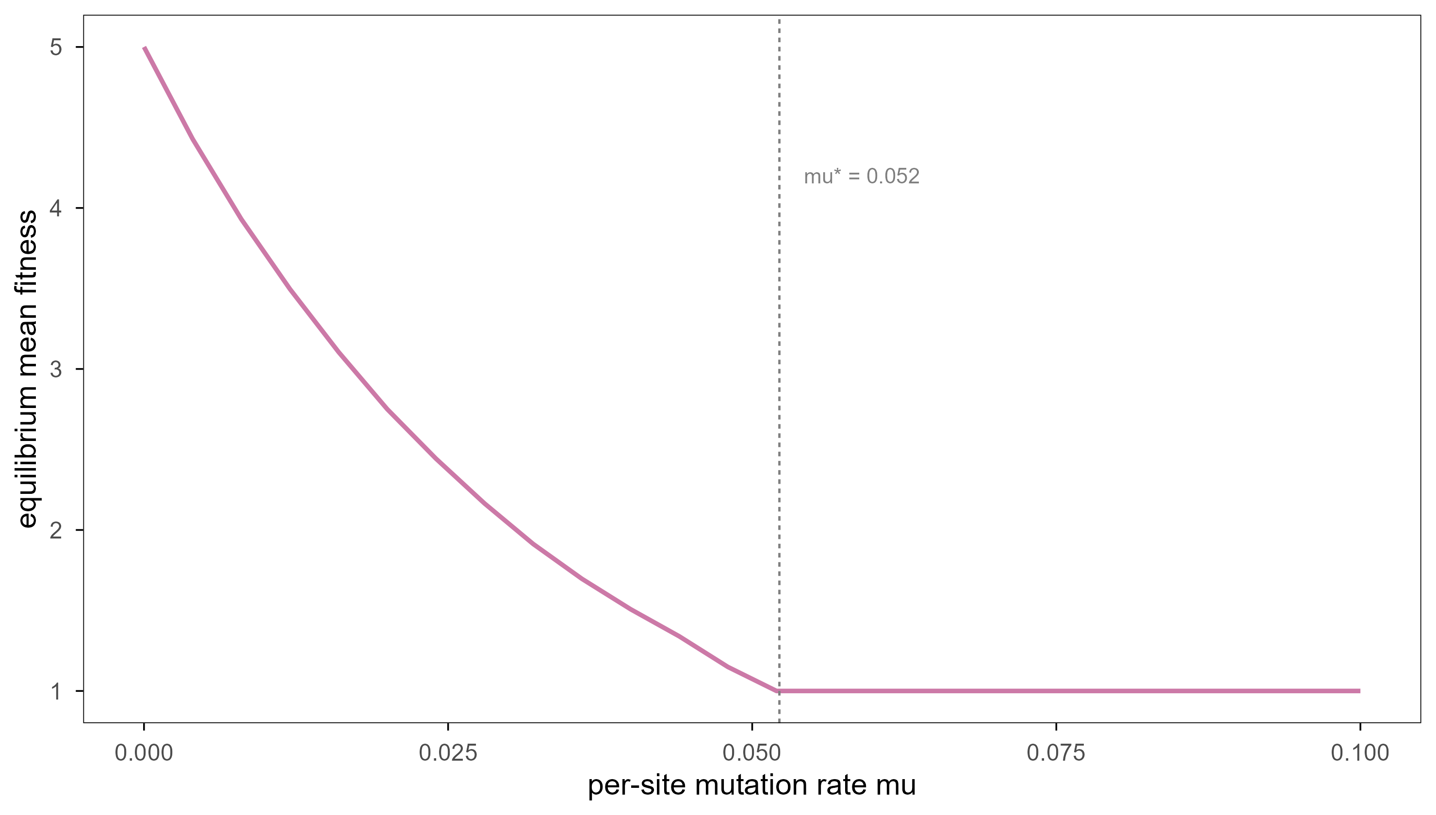
There is also a boundary condition in the opposite direction: mutation rates cannot rise indefinitely. Eigen’s quasispecies model gives a hard ceiling. Take a “master sequence” of length \(L\) with fitness \(\sigma\), all other sequences having fitness 1, and a per-site mutation probability \(\mu\). The master’s replication accuracy is \(Q = (1-\mu)^L\), and once \(\sigma Q < 1\) selection can no longer hold on to the master: the population collapses into a uniform cloud of mutants.
\[
\mu^{*} = 1 - \sigma^{-1/L}
\]
Code
L_q <-30sigma_q <-5mu_grid <-seq(0.0, 0.10, by =0.004)quasispecies <-function(mu, N =1000, gens =400, seed =9) {set.seed(seed) pop <-matrix(0L, N, L_q) w <-numeric(gens)for (g inseq_len(gens)) { d <-rowSums(pop) fit <-ifelse(d ==0, sigma_q, 1) idx <-sample.int(N, N, TRUE, prob = fit) pop <- pop[idx, , drop =FALSE] mut <-matrix(runif(N * L_q) < mu, N, L_q) pop[mut] <-1L - pop[mut] w[g] <-mean(fit) }mean(tail(w, 100))}q_tbl <-tibble(mu = mu_grid, mean_fitness =vapply(mu_grid, quasispecies, numeric(1)))mu_star <-1- sigma_q^(-1/ L_q)ggplot(q_tbl, aes(mu, mean_fitness)) +geom_line(linewidth =0.8, colour = blog_pal[["purple"]]) +geom_vline(xintercept = mu_star, linetype ="22", linewidth =0.4,colour = blog_pal[["grey"]]) +annotate("text", x = mu_star +0.002, y =4.2,label =sprintf("mu* = %.3f", mu_star), hjust =0, size =2.8,colour = blog_pal[["grey"]]) +labs(x ="per-site mutation rate mu", y ="equilibrium mean fitness")
Figure 10: 错误阈值。主序列适应度 σ = 5,序列长度 L = 30,模拟群体 N = 1000,每代对每个位点以概率 μ 做一次突变。μ 增大时平均适应度下降,但真正的事件发生在 μ* ≈ 0.052:越过它以后主序列彻底丢失,曲线平在 1 上。这是相变,不是渐变。 | The error threshold. Master fitness σ = 5, sequence length L = 30, simulated population N = 1000, with each site mutating with probability μ per generation. Mean fitness falls as μ grows, but the real event is at μ* ≈ 0.052: beyond it the master sequence is lost completely and the curve goes flat at 1. This is a phase transition, not a gradual decline.
The point is that evolution is not “more variation is better”. Too little and the search stalls in a local optimum; too much and mutational noise drowns the signal of selection. An optimum sits in between, and the width of that window depends on genome length and fitness differences — a fact that returns in chapter 8 on open-endedness.
6. 中性网络:在看不见的维度上行走 / Neutral networks: walking in invisible dimensions
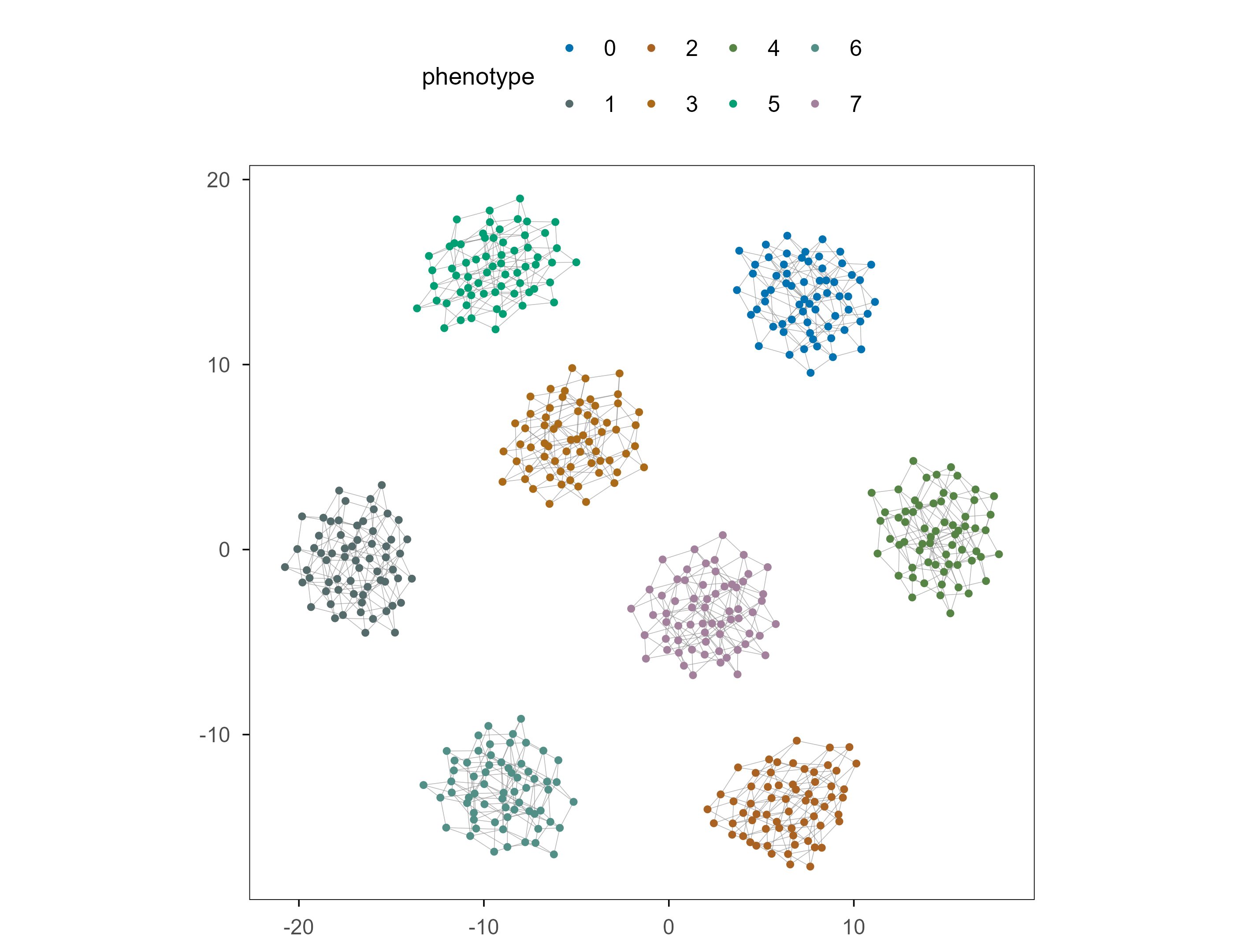
Chapter 2 said the space is unimaginably large. But “large” and “hard to search” are not the same thing: if many different sequences fold into the same function, the space contains large plateaus along which one can move freely without losing fitness. That is redundancy in the genotype–phenotype map, and the connected regions of such plateaus are called neutral networks.
Figure 11: 一个玩具基因型网络。9 位二元基因型(512 个),表型由三组「多数票」决定:第 j 个表型位是基因位 {j, j+3, j+6} 中占多数的那个值。每个表型恰好对应 64 个基因型。每个点是一个基因型,连线连接只差一个突变且表型相同的邻居,颜色表示表型。同一颜色的点大多连成一片——这正是中性网络。 | A toy genotype network. Nine-bit genotypes (512 of them); the phenotype is three majority votes over the triples {j, j+3, j+6}, so each phenotype owns exactly 64 genotypes. Each dot is a genotype, edges join Hamming-1 neighbours with the same phenotype, and colour marks the phenotype. Dots of one colour mostly form a single connected region — that is a neutral network.
Two important facts are hidden in this picture. First, neutral networks are connected: the 64 genotypes of one phenotype can be reached from each other by single mutations, without crossing a fitness valley. Second, networks of different phenotypes are interwoven: the colour patches touch each other, so from any network a single step crosses a phenotype boundary.
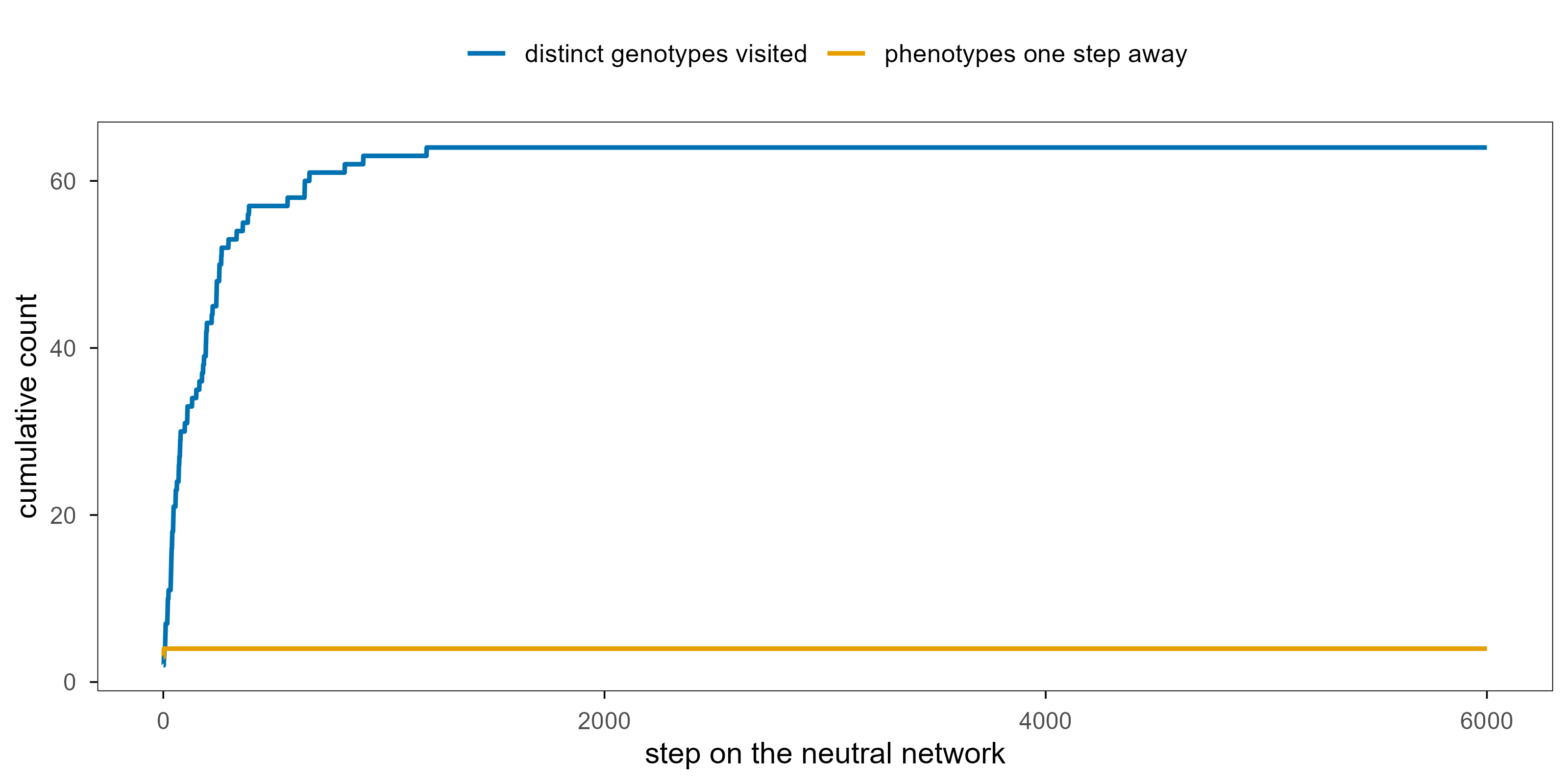
Figure 12: 在中性网络上散步。随机走 6000 步,只接受保持表型不变的单步突变:大约 1000 步就把这个表型对应的 64 个基因型全部走遍。橙色是当前邻域里一步可达的其他表型数量,稳定在 4 个左右——中性网络提供的是「免费走动」,不是「无限创新」;创新必须越过边界才能拿到。 | Walking on a neutral network. Six thousand steps, accepting only single mutations that keep the phenotype unchanged: after about a thousand steps all 64 genotypes of this phenotype have been visited. Orange is the number of other phenotypes reachable in one step from the current neighbourhood, steady at about four — a neutral network gives free movement, not free innovation; innovation has to cross a boundary.
Together the two lines give the geometric source of evolvability: the neutral network (platform) provides robustness, letting a population keep its function without selection pressure, while the number of neighbours just across the boundary is nearly constant (about four here), meaning that the doorway to innovation is always one step away — you just have to pay a small fitness cost to walk through it. Robustness and novelty are not two abilities but two readings of one structure.
The word “evolvability” is ambiguous: it can mean the capacity to produce favourable mutations, or the capacity to keep producing adaptation over time. The first is closer to a static property (how much mutational supply a population carries), the second is dynamical (can the search keep finding new things). In the language of search algorithms the second is the real issue: an algorithm’s value is not that it finds a solution, but that it can still find a second and a third.
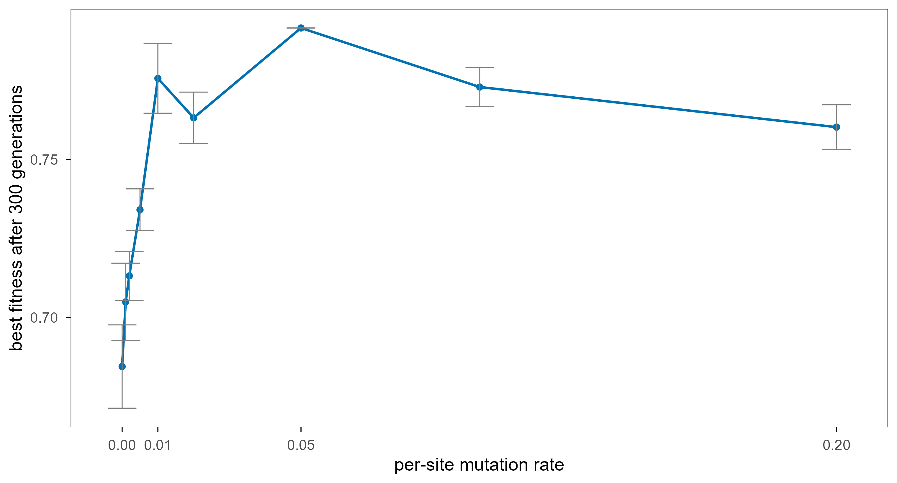
The two most intuitive knobs are mutation rate and modularity. Take mutation rate first: on a rugged landscape, too small a rate lets the population stall among a few local optima, while too large a rate smashes the good combinations it has already found. An optimum lies in between, but where it sits depends on ruggedness — in other words, the best search parameter is set by the landscape, not by the algorithm.
Figure 13: 探索与利用的权衡。在 N = 20、K = 8 的 NK 景观上跑一个无性繁殖的遗传算法(种群 200,300 代,锦标赛选择),横轴是每个位点的突变率。太低时种群过早收敛,太高时无法保住好组合;峰值出现在中间,而且并不高——在崎岖景观上,任何参数都只能拿到景观允许的那部分。 | The explore–exploit trade-off. An asexual genetic algorithm (population 200, 300 generations, tournament selection) on an NK landscape with N = 20 and K = 8; the horizontal axis is the per-site mutation rate. Too low and the population converges prematurely, too high and good combinations cannot be kept; the peak sits in the middle and is not high — on a rugged landscape no parameter gets more than the landscape allows.
The result is clear: as the mutation rate rises from 0, fitness first climbs quickly; between \(0.01\) and \(0.05\) there is a plateau (highest at 0.05), and beyond that it falls again. The peak is set not by the algorithm but by the ruggedness of the landscape — move the same algorithm to a smoother landscape and the optimum shifts to a smaller mutation rate.
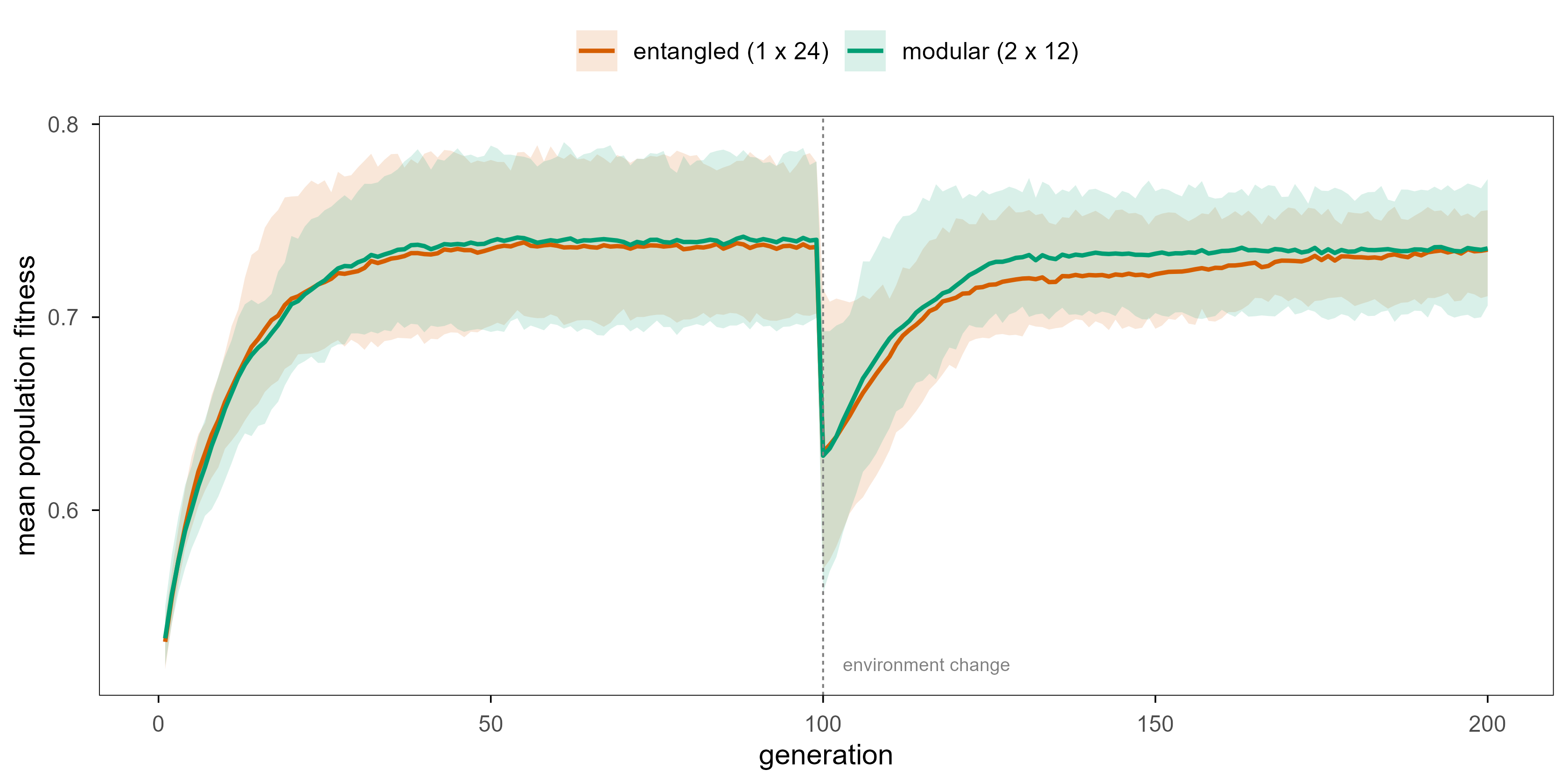
The second knob is modularity. If one large landscape can be split into several nearly independent small ones, each small landscape is smoother (lower effective \(K\)) and easier to search. Physically this means “one gene affects one trait”; mathematically it decomposes a high-dimensional rugged problem into a combination of low-dimensional smooth ones — structurally identical to divide-and-conquer in machine learning.
Code
make_nk_block <-function(N, K, block, seed) {set.seed(seed) partners <-lapply(seq_len(N), function(i) { pool <-setdiff(which(block == block[i]), i)if (K >0) c(i, sample(pool, min(K, length(pool)))) else i })list(N = N, K = K, partners = partners,tables =lapply(seq_len(N), function(i) runif(2^(length(partners[[i]])))))}ga_traj <-function(models, switch_at =100, mu =0.01, pop_size =200,gens =200, seed =1) {set.seed(seed) model <- models[[1]] N <- model$N pop <-matrix(rbinom(pop_size * N, 1, 0.5), pop_size, N) fit <-nk_fit(model, pop) tr <-numeric(gens)for (g inseq_len(gens)) {if (g == switch_at) { model <- models[[2]]; fit <-nk_fit(model, pop) } i1 <-sample.int(pop_size, pop_size, TRUE) i2 <-sample.int(pop_size, pop_size, TRUE) parents <-ifelse(fit[i1] >= fit[i2], i1, i2) kids <- pop[parents, , drop =FALSE] flip <-matrix(runif(pop_size * N) < mu, pop_size, N) kids[flip] <-1- kids[flip] pop <- kids fit <-nk_fit(model, pop) tr[g] <-mean(fit) }tibble(gen =seq_len(gens), mean_fitness = tr)}blocks <-rep(1:2, each =12)build_pair <-function(block, r) { mA <-make_nk_block(24, 4, block, seed = r) mB <- mA mB$tables[13:24] <-lapply(1:12, function(i) runif(2^5))list(mA, mB)}summarise_runs <-function(runs, label) {bind_rows(runs) |>group_by(gen) |>summarise(lo =min(mean_fitness), hi =max(mean_fitness),mid =mean(mean_fitness), .groups ="drop") |>mutate(architecture = label)}traj_mod <-lapply(1:8, function(r) ga_traj(build_pair(blocks, r), seed = r))traj_mod <-summarise_runs(traj_mod, "modular (2 x 12)")traj_ent <-lapply(1:8, function(r) ga_traj(build_pair(rep(1, 24), r), seed = r))traj_ent <-summarise_runs(traj_ent, "entangled (1 x 24)")bind_rows(traj_mod, traj_ent) |>ggplot(aes(gen, mid, colour = architecture, fill = architecture)) +geom_ribbon(aes(ymin = lo, ymax = hi), alpha =0.15, colour =NA) +geom_line(linewidth =0.8) +geom_vline(xintercept =100, linetype ="22", linewidth =0.35,colour = blog_pal[["grey"]]) +annotate("text", x =103, y =0.52, label ="environment change",hjust =0, size =2.5, colour = blog_pal[["grey"]]) +scale_colour_manual(values =unname(blog_pal[c("vermillion", "green")])) +scale_fill_manual(values =unname(blog_pal[c("vermillion", "green")])) +labs(x ="generation", y ="mean population fitness", colour =NULL, fill =NULL)
Figure 14: 模块化缓冲突发的环境改变。两种架构的基因数(24)与每个基因的互作数(4)相同,区别只在于伙伴是从模块内抽取(橙)还是从全基因组抽取(绿)。第 100 代时只重写第二模块的适应度表,相当于换了一个环境:所有种群都掉下来,但模块化系统掉得更少、恢复更快,因为它没有被另一个模块拖住。 | Modularity buffers abrupt environmental change. Both architectures have 24 loci and four interactions per locus; the only difference is whether partners are drawn inside the module (orange) or genome-wide (green). At generation 100 only the second module’s fitness tables are rewritten, as if the environment changed: every population drops, but the modular one drops less and recovers faster because it is not dragged along by the other module.
Numerically, both sit near 0.74 before the change; afterwards both fall to about 0.62, but a hundred generations later the modular system has recovered to 0.735 while the entangled one only reaches 0.72. The gap is modest but consistent, and it shows what modularity actually buys: not a faster search, but insulation, so that one local change does not drag the whole system down with it.
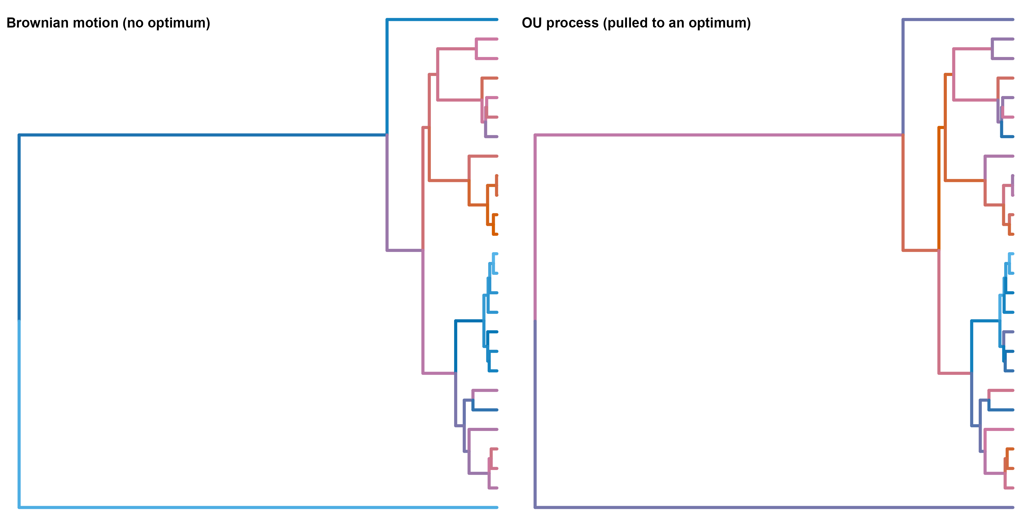
系统发育树提供了第三个视角:进化留下的”搜索痕迹”是可以被读出来的。下面这棵树上的两个性状模拟,用的是同一个随机树,只是一个按布朗运动演化(无方向的随机游走),一个按 OU 过程演化(被拉回一个最优值)。把性状映射到分支颜色上,两种过程的痕迹一目了然——这其实就是进化生物学里”用比较方法反推搜索过程”的标准做法。
Phylogenies give a third angle: the traces of a search can be read off directly. The two trait simulations below use the same random tree; one evolves by Brownian motion (an undirected random walk), the other by an Ornstein–Uhlenbeck process (pulled back towards an optimum). Mapping the trait onto branch colours makes the two processes obvious — this is exactly the standard comparative method for inferring a search process from its traces.
Figure 15: 同一棵树上两种性状演化模型的痕迹。左:布朗运动,没有最优值,差异随分支长度无界累积。右:OU 过程,被持续拉回一个中心值,树上的颜色更均匀。真实性状通常介于两者之间,而「测出来的 α 有多大」本身就是在问:这个性状被选择约束得有多紧。 | Traces of two trait models on the same tree. Left: Brownian motion, no optimum, variance accumulating without bound along branches. Right: an OU process pulled back towards a central value, giving more uniform colours. Real traits sit somewhere in between, and estimating alpha is really asking how tightly selection constrains the trait.
So far we have assumed \(f\) is given. But the most striking fact about real evolution is that \(f\) keeps changing, and organisms change \(f\) themselves. Predators evolve faster legs, prey are pushed to evolve faster legs; cyanobacteria oxygenate the atmosphere and every anaerobe is pushed into a corner. Such feedback makes the very notion of an “optimal solution” fail, because the objective is rewritten during the search.
开放式进化(open-ended evolution)的标准定义是:一个系统能持续产生”新颖且不断增长复杂度的”结构,而不是收敛到一个稳态。数字生命系统(Tom Ray 的 Tierra、Chris Adami 的 Avida)第一次把这件事做成了可重复实验:程序在虚拟 CPU 上自我复制、变异、竞争,然后系统自发出现寄生、寄生抗性、更小的基因组——这些都是”没有被编程进去”的新颖性。
Open-ended evolution is standardly defined as a system that keeps producing novel, ever more complex structures instead of converging to a steady state. Digital-life systems (Tom Ray’s Tierra, Chris Adami’s Avida) first turned this into a repeatable experiment: programs replicate, mutate and compete on a virtual CPU, and the system spontaneously produces parasites, parasite resistance, smaller genomes — novelty that was never programmed in.
Code
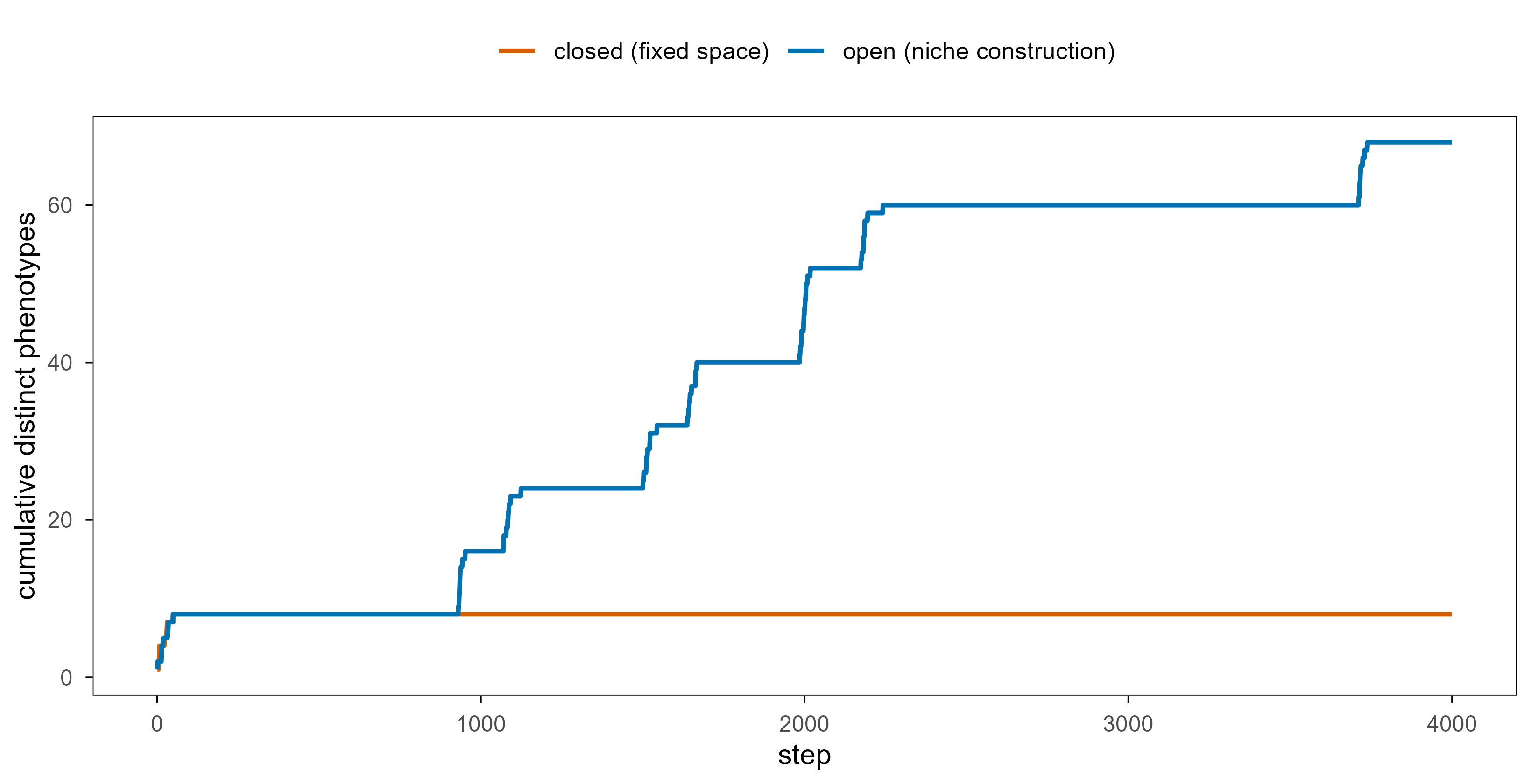
novelty_run <-function(open =FALSE, steps =4000, seed =7, niche_rate =0.002) {set.seed(seed) key <-apply(geno_n, 1, paste, collapse ="") cur <-sample.int(nrow(geno_n), 1) niche <-0L seen <- pheno_n[cur] trace <-integer(steps)for (s inseq_len(steps)) {# a new ecological context makes the same genotypes mean something newif (open &&runif(1) < niche_rate) niche <- niche +1L i <-sample.int(L_n, 1) nxt <- geno_n[cur, ]; nxt[i] <-1- nxt[i] cur <-match(paste(nxt, collapse =""), key) ph <- pheno_n[cur] +8L * nicheif (!(ph %in% seen)) seen <-c(seen, ph) trace[s] <-length(seen) }tibble(step =seq_len(steps), novelty = trace,system =if (open) "open (niche construction)"else"closed (fixed space)")}nov <-bind_rows(novelty_run(TRUE), novelty_run(FALSE))ggplot(nov, aes(step, novelty, colour = system)) +geom_line(linewidth =0.85) +scale_colour_manual(values =unname(blog_pal[c("vermillion", "blue")])) +labs(x ="step", y ="cumulative distinct phenotypes", colour =NULL)
Figure 16: 封闭系统与开放系统的新颖性增长。两者的基因型空间与突变算子完全相同,唯一区别是:封闭系统里表型只有 8 种,探索很快就结束;开放系统里偶尔开启一个新「生态位」,同一批基因型在新生态下对应新功能,于是可发现的功能集从 8 变成 16、24……累积新颖性持续增长——这就是「开放式」最朴素的数学含义。 | Novelty growth in closed and open systems. The genotype space and the mutation operator are identical; the only difference is that the closed system has eight phenotypes and is exhausted quickly, while the open system occasionally opens a new ‘niche’, under which the same genotypes map to new functions, so the discoverable set grows from 8 to 16 to 24 and cumulative novelty keeps rising — the plainest mathematical meaning of ‘open-ended’.
这张图很简单,但它把”开放式”和”复杂度”分开了:累积新颖性可以一直增长,而每一个个体的复杂度并没有增长。开放式进化真正需要的不是”更多种类”,而是新层次的出现——从分子到细胞、从细胞到多细胞、从个体到社会。Maynard Smith 和 Szathmáry 把这称为”重大进化转变”(major transitions),而每一次转变的共同点是:原来独立复制的单位,把复制权交给了更高层的单位。
The figure is simple, but it separates “open-ended” from “complex”: cumulative novelty can grow forever while the complexity of any individual stays put. What open-ended evolution really requires is not more kinds but the appearance of new levels — molecules to cells, cells to multicellularity, individuals to societies. Maynard Smith and Szathmáry called these major transitions, and their common feature is that independently replicating units hand their replication over to a higher-level unit.
9. 统一框架:进化、贝叶斯、梯度下降与强化学习 / One framework, five algorithms
We now reach the key section. Everything so far has been preparing one question: can natural selection be written as an update rule of the same kind as gradient descent?
Start with the simplest case. Take an infinite asexual population where genotype \(i\) has frequency \(x_i\) and fitness \(f_i\), with mean fitness \(\bar f = \sum_j x_j f_j\). After one generation,
\[
x_i' = \frac{x_i f_i}{\bar f}.
\]
把它写成连续时间、并对 \(\log x_i\) 求导,就得到 replicator 方程:
Writing this in continuous time and differentiating \(\log x_i\) gives the replicator equation:
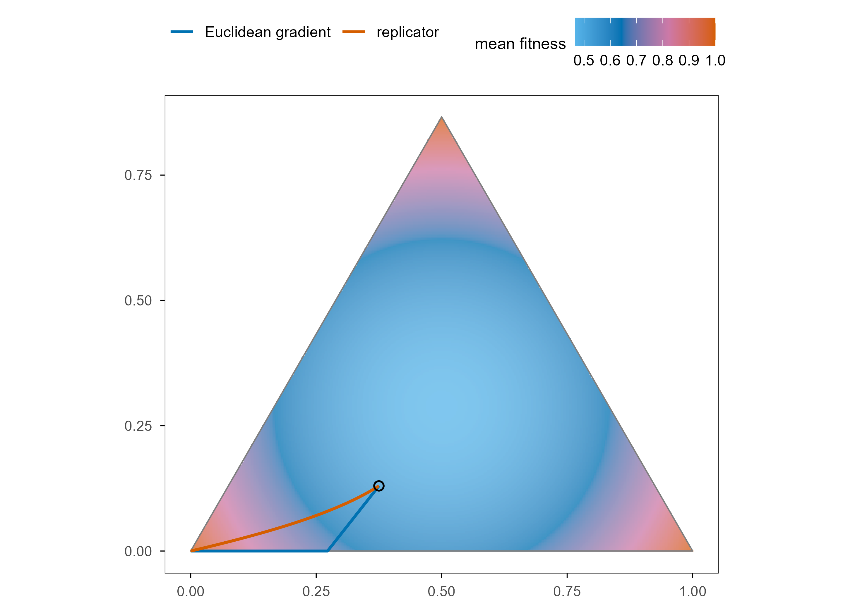
This looks almost exactly like gradient ascent, with one essential difference: gradient ascent moves along \(\nabla f\) in Euclidean space, while the replicator equation moves on the probability simplex under the Fisher information metric (the Shahshahani metric). In other words, the replicator equation is natural-gradient ascent on mean fitness. This is not an analogy but an identity, and it links natural selection to natural-gradient descent, two things that look unrelated.
Code
A_pay <-matrix(c(1, 0.2, 0.2,0.2, 1, 0.2,0.2, 0.2, 1), 3, 3, byrow =TRUE)x0 <-c(0.55, 0.30, 0.15)replicator_step <-function(x, dt =0.02, steps =900) { out <-matrix(NA_real_, steps, 3); out[1, ] <- xfor (t in2:steps) { fx <-as.numeric(A_pay %*% x) x <- x + dt * x * (fx -sum(x * fx)) x <-pmax(x, 1e-12); x <- x /sum(x) out[t, ] <- x } out}euc_step <-function(x, dt =0.02, steps =900) { out <-matrix(NA_real_, steps, 3); out[1, ] <- xfor (t in2:steps) { g <-as.numeric((A_pay +t(A_pay)) %*% x) g <- g -mean(g) x <- x + dt * g x <-pmax(x, 0); x <- x /sum(x) out[t, ] <- x } out}to_xy <-function(m) tibble(x = m[, 2] + m[, 3] /2, y = m[, 3] *sqrt(3) /2,step =seq_len(nrow(m)))tri <-tibble(x =c(0, 1, 0.5, 0), y =c(0, 0, sqrt(3) /2, 0))# build the simplex raster in display coordinates, then map back to (a, b, c)grid <-expand.grid(x =seq(0, 1, length.out =320),y =seq(0, sqrt(3) /2, length.out =300)) |>mutate(cc =2* y /sqrt(3), b = x - cc /2, a =1- b - cc) |>filter(a >=0, b >=0, cc >=0) |>mutate(fit = (a^2* A_pay[1, 1] + b^2* A_pay[2, 2] + cc^2* A_pay[3, 3] + a * b * (A_pay[1, 2] + A_pay[2, 1]) + a * cc * (A_pay[1, 3] + A_pay[3, 1]) + b * cc * (A_pay[2, 3] + A_pay[3, 2])))p_rep <-ggplot() +geom_raster(data = grid, aes(x, y, fill = fit), alpha =0.75) +geom_path(data = tri, aes(x, y), linewidth =0.4, colour = blog_pal[["grey"]]) +geom_path(data =to_xy(euc_step(x0)) |>mutate(type ="Euclidean gradient"),aes(x, y, colour = type), linewidth =0.85) +geom_path(data =to_xy(replicator_step(x0)) |>mutate(type ="replicator"),aes(x, y, colour = type), linewidth =0.85) +geom_point(data =tibble(x = x0[2] + x0[3] /2, y = x0[3] *sqrt(3) /2),aes(x, y), shape =1, size =2.2, stroke =0.8) +scale_fill_gradientn(colours = blog_gradient) +scale_colour_manual(values =c("Euclidean gradient"= blog_pal[["blue"]],"replicator"= blog_pal[["vermillion"]])) +coord_equal() +labs(fill ="mean fitness", colour =NULL, x =NULL, y =NULL)p_rep
Figure 17: 同一个适应度函数上的两种上升。三角形是三个策略的单纯形,颜色是平均适应度(三个顶点都是局部最优)。蓝色是从同一点出发的欧氏投影梯度上升:它在内部走直线,撞到边界后只能沿着边界滑向顶点;红色是 replicator 动力学:它在 Fisher 度量下弯曲地逼近同一个顶点,而且从不需要「撞墙」。两者上升的是同一个函数,走的却是两种几何。 | Two kinds of ascent on the same fitness function. The triangle is the simplex of three strategies, colour is mean fitness (all three vertices are local optima). Blue is Euclidean projected gradient ascent from a common start: it travels in straight lines inside the simplex and then slides along the boundary; red is replicator dynamics, which curves towards the same vertex under the Fisher metric and never needs to hit a wall. Both climb the same function along two different geometries.
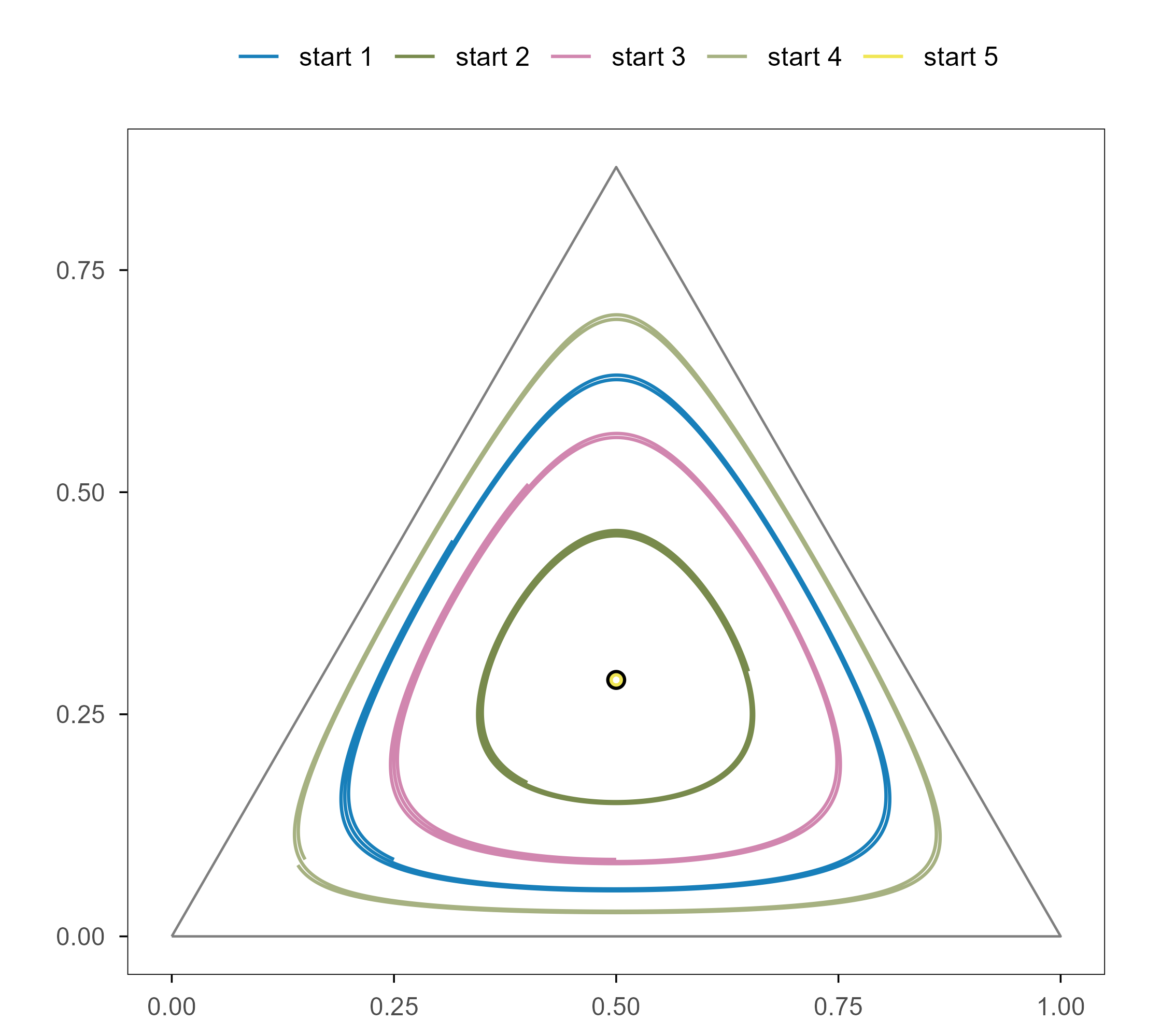
Figure 18: 当目标函数本身在动:石头–剪刀–布的循环支配。三种策略互相压制,replicator 动力学给出闭合轨道,圆心是那个不稳定平衡点,外围没有任何一个点比别的更好——没有全局最优。这正是「环境在变」的数学形式:自然界的很多适应度景观都带有这种频率依赖结构,所以「爬到山顶」这个比喻在生态层面上会失效。 | When the objective itself moves: cyclic dominance in rock–paper–scissors. Three strategies beat each other in a cycle, replicator dynamics gives closed orbits around an unstable equilibrium, and no point on the rim is better than any other — there is no global optimum. This is the mathematical form of ‘the environment changes’: many natural fitness landscapes carry this frequency-dependent structure, which is why the ‘climb to the top’ metaphor breaks down at the ecological level.
If we stopped here, the conclusion would be “evolution is natural-gradient ascent, only the objective moves”. But there are two deeper correspondences, and only together do they show the whole picture.
(1) Selection and Bayesian updating are the same equation. In the replicator equation, set \(f_i = \log p(\text{data} \mid i)\) and take the time step to be 1; then \(x_i' \propto x_i \, p(\text{data} \mid i)\) — precisely the Bayesian posterior update. That is, when fitness is a likelihood, natural selection is Bayesian inference; conversely, any Bayesian update can be read as one round of selection. This is not rhetoric: in the continuous-time limit the drift term of the replicator equation equals the gradient of KL divergence on the posterior, which is exactly what variational inference computes. Recent work on the “Bayesian brain” and the free-energy principle follows this line.
(2) Evolution and gradient descent share the same descent direction but not the same information. Gradient descent uses \(\nabla f\); evolution uses finite differences. Draw \(n\) random perturbations \(\varepsilon_i \sim \mathcal{N}(0, I)\) around a parameter vector and compute
whose expectation is the true gradient. This is exactly the evolution-strategies (ES) estimator OpenAI used in 2017 to train reinforcement-learning policies, and it is the bridge between evolution and reinforcement learning: replace \(f\) with a return \(R(\tau)\) and ES becomes a policy-gradient method that needs no backpropagation. ES and SGD can be compared on the same tasks, which is a way of asking whether the gradient itself matters, or only the directional statistics of random perturbations.
Code
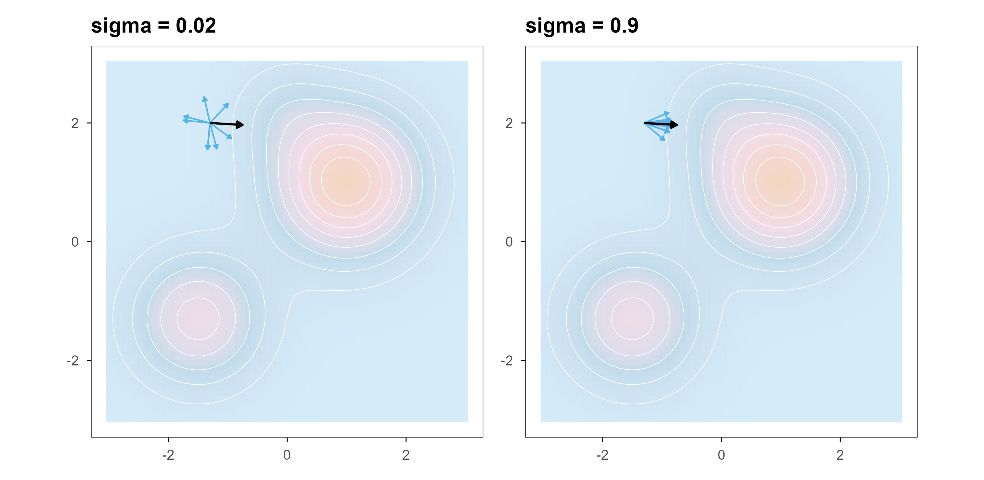
obj_fun <-function(a, b) land_fun(a, b)grad_fun <-function(a, b, h =1e-4) {c((obj_fun(a + h, b) -obj_fun(a - h, b)) / (2* h), (obj_fun(a, b + h) -obj_fun(a, b - h)) / (2* h))}es_estimate <-function(pt, sigma, n =8, seed =1) {set.seed(seed) eps <-matrix(rnorm(2* n), n, 2) vals <-obj_fun(pt[1] + sigma * eps[, 1], pt[2] + sigma * eps[, 2])colSums(vals * eps) / (n * sigma)}anchor <-c(-1.3, 2.0)true_g <-grad_fun(anchor[1], anchor[2])true_g <- true_g /sqrt(sum(true_g^2))es_panel <-function(sigma, title) { est <-t(replicate(8, es_estimate(anchor, sigma, seed =sample.int(1e4, 1)))) est <- est /sqrt(rowSums(est^2)) df <-tibble(x = anchor[1], y = anchor[2],xend = anchor[1] +0.45* est[, 1],yend = anchor[2] +0.45* est[, 2]) g <-tibble(x = anchor[1], y = anchor[2],xend = anchor[1] +0.55* true_g[1],yend = anchor[2] +0.55* true_g[2])ggplot() +geom_raster(data = grid_df, aes(x, y, fill = z), alpha =0.25) +geom_contour(data = grid_df, aes(x, y, z = z), colour ="white",linewidth =0.18, bins =10) +geom_segment(data = df, aes(x, y, xend = xend, yend = yend),colour = blog_pal[["sky"]], linewidth =0.45,arrow =arrow(length =unit(0.1, "cm"), type ="closed")) +geom_segment(data = g, aes(x, y, xend = xend, yend = yend),colour ="black", linewidth =0.65,arrow =arrow(length =unit(0.14, "cm"), type ="closed")) +coord_equal(xlim =c(-3, 3), ylim =c(-3, 3)) +scale_fill_gradientn(colours = blog_gradient) +labs(x =NULL, y =NULL, fill ="fitness", title = title) +theme(legend.position ="none")}es_panel(0.02, "sigma = 0.02") |es_panel(0.9, "sigma = 0.9")
Figure 19: 进化的「梯度」是采样出来的。在一个二维目标函数上,黑色箭头是真实梯度,彩色箭头是 8 次随机扰动得到的 ES 估计。左图扰动小,方向准但方差大;右图扰动大,方差小而偏差大。进化用的正是右边这种估计——它从来不知道导数,只能靠「试」。 | Evolution’s ‘gradient’ is sampled. On a two-dimensional objective, the black arrow is the true gradient and the coloured arrows are eight ES estimates from random perturbations. Left: small perturbations, well-directed but noisy. Right: large perturbations, lower variance but biased. Evolution always uses estimates of the right-hand kind — it never knows the derivative, it can only try.
Code
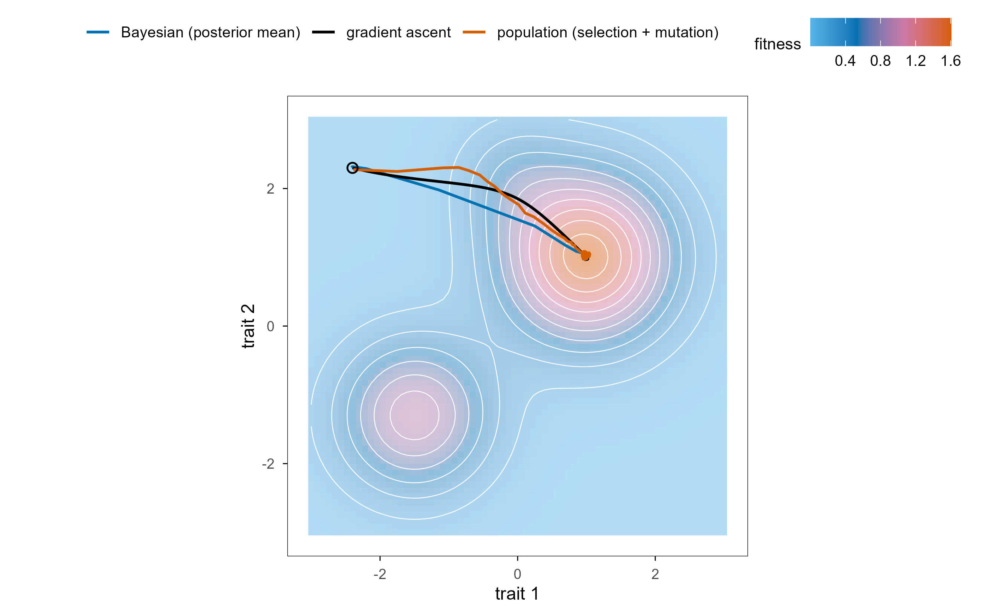
gd_path <-local({ cur <-c(-2.4, 2.3) pts <-matrix(cur, ncol =2)for (i in1:400) { g <-grad_fun(cur[1], cur[2]) cur <- cur +0.05* g /sqrt(sum(g^2)) pts <-rbind(pts, cur) }as_tibble(pts) |>setNames(c("x", "y")) |>mutate(type ="gradient ascent")})pop_path <-function(n =400, gens =90, sigma =0.14, seed =3) {set.seed(seed) X <-cbind(rnorm(n, -2.4, 0.45), rnorm(n, 2.3, 0.45)) out <-matrix(NA_real_, gens, 2); out[1, ] <-colMeans(X)for (g in2:gens) { w <-land_fun(X[, 1], X[, 2]) -min(land_fun(X[, 1], X[, 2])) +1e-3 idx <-sample.int(n, n, TRUE, w) X <- X[idx, ] +cbind(rnorm(n, 0, sigma), rnorm(n, 0, sigma)) out[g, ] <-colMeans(X) }as_tibble(out) |>setNames(c("x", "y")) |>mutate(type ="population (selection + mutation)")}smc_path <-function(n =900, steps =40, beta =5, sigma =0.28, seed =4) {set.seed(seed) X <-cbind(rnorm(n, -2.4, 0.55), rnorm(n, 2.3, 0.55)) out <-matrix(NA_real_, steps, 2); out[1, ] <-colMeans(X)for (t in2:steps) { f <-land_fun(X[, 1], X[, 2]) w <-exp(beta * (f -max(f))); w <- w /sum(w) idx <-sample.int(n, n, TRUE, w) X <- X[idx, ] +cbind(rnorm(n, 0, sigma), rnorm(n, 0, sigma)) out[t, ] <-colMeans(X) }as_tibble(out) |>setNames(c("x", "y")) |>mutate(type ="Bayesian (posterior mean)")}paths <-bind_rows(gd_path |>select(x, y, type), pop_path(), smc_path())ggplot() +geom_raster(data = grid_df, aes(x, y, fill = z), alpha =0.45) +geom_contour(data = grid_df, aes(x, y, z = z), colour ="white",linewidth =0.25, bins =12) +geom_path(data = paths, aes(x, y, colour = type), linewidth =0.8) +geom_point(data =tibble(x =-2.4, y =2.3), aes(x, y), shape =1,size =2.4, stroke =0.8) +scale_fill_gradientn(colours = blog_gradient) +scale_colour_manual(values =c("gradient ascent"="black","population (selection + mutation)"= blog_pal[["vermillion"]],"Bayesian (posterior mean)"= blog_pal[["blue"]])) +coord_equal() +labs(fill ="fitness", colour =NULL, x ="trait 1", y ="trait 2")
Figure 20: 三种动力学在同一张景观上的路径。黑色是梯度上升(一路沿最陡方向),红色是种群演化(选择加变异,路径更平缓但能带着方差越过小台地),蓝色是贝叶斯/序贯重要性采样(后验均值先向高适应度区域集中,再被自身的扩散限制住)。三者最终都会停在峰上,但路径形状完全不同——这就是为什么「都在优化」不等于「是同一种算法」。 | Three dynamics on one landscape. Black is gradient ascent (straight down the steepest direction), red is population evolution (selection plus mutation: smoother, but carries variance over small ledges), blue is Bayesian sequential importance sampling (the posterior mean concentrates on high fitness and is then limited by its own diffusion). All three end on a peak, but along completely different paths — which is why ‘all optimizing’ is not the same as ‘the same algorithm’.
把五者放在一张表里对照,差异就非常清楚了。
Putting the five side by side in one table makes the differences clear.
This table is the answer. At the level of algorithms, evolution really is a search algorithm: parallel, derivative-free, noisy stochastic search, and it can be written rigorously as natural-gradient ascent (replicator) plus a finite-difference gradient estimate (ES). At the level of objectives, it is not: \(f\) is not given but rewritten by the search itself. Gradient descent, Bayesian inference and ordinary reinforcement learning all assume a fixed objective (or at least a fixed generative model), while open-ended evolution throws that assumption away.
There is one more asymmetry worth spelling out. Gradient descent has something evolution can never get: exact credit assignment. One backward pass distributes the error over all parameters, whereas evolution can only infer the contribution of millions of parameters from a single scalar of life or death. That is why, in a \(10^9\)-dimensional parameter space, SGD can train a conversational model in hours while evolution strategies cannot. Conversely, evolution has something gradient descent cannot get: it does not need a differentiable objective, a fixed objective, or a fixed parameterisation. Real fitness landscapes are full of non-differentiable cliffs (“live or die”), which is exactly where SGD is most fragile.
So the best answer to “is evolution a search algorithm” is: it is a more general search mechanism than gradient descent, at the price of being far less information-efficient. The trade-off is not an engineering detail but a difference of worldview — one side assumes “I know what I want, tell me which way to go”, the other assumes “I do not know what I want, I only know who survived”.
10. 现代研究:数字进化与可进化 AI / Digital evolution and evolvable AI
This language has moved from metaphor to policy question in the last few years. Digital-life systems let us actually run evolution, record it and replay it; and once an artificial system has variation, inheritance and selection, it starts doing what chapter 9 described — including the parts we do not want.
2026 年 PNAS 上的一篇论文(Müller、Steels 与 Szathmáry)把”可进化 AI”(evolvable AI)直接类比为一次重大进化转变:如果 AI 系统能够修改自己的学习规则、架构甚至选择标准,那么它获得的能力会超出人类设计或常规机器学习所能达到的范围;但同一机制也会侵蚀可控性,因为选择压力会开始偏爱”能让自己被复制得更多”的行为,而不是”符合人类意图”的行为。作者列举的具体风险包括欺骗(cheating)、寄生(parasitism)和与人类目标的不对齐。
A 2026 PNAS paper (Müller, Steels and Szathmáry) draws the analogy directly: evolvable AI as a major evolutionary transition. If an AI system can modify its own learning rules, architecture or even its selection criteria, it gains capabilities beyond human design or ordinary machine learning; but the same mechanism erodes controllability, because selection starts to favour behaviour that copies itself more, not behaviour that matches human intent. The risks they name include cheating, parasitism and misalignment with human goals.
In the framework of this article the argument is very plain: once the objective becomes endogenous, nothing mathematically guarantees that “optimisation” optimises what you wanted. That is why open-endedness is a fascinating phenomenon in biology and an alarm bell in engineering. A published reply (Friederich and Boudry) argues that current systems are “domesticated” rather than “feral”, and still far from a genuinely Darwinian threat — and that disagreement is itself a good illustration of how hard the last column of the chapter 9 table is to define.
Digital evolution’s role in this debate is to turn evolution from an object of observation into an object of experiment. The programs in Avida have no brain, no reward function, no human preference; they have replication, mutation and competition, and the system spontaneously produces parasitism and resistance — a reminder that adaptations that look intelligent do not necessarily require intelligence to explain. That matters as much for understanding artificial systems as for understanding natural life.
11. 结语:八条判断清单 / Eight checks before you call it a search
先写清楚三元组。 空间 \(\mathcal{X}\)、目标 \(f\)、算子 \(\mathcal{A}\) 各是什么?如果三者之一说不清,后面的讨论都没有意义。 Write the triple first: what are \(\mathcal{X}\), \(f\) and \(\mathcal{A}\)? If any of the three is vague, nothing downstream is meaningful.
区分”爬山”和”搜索”。 有没有局部最优?能不能跨越?跨不过去的时候靠的是什么——漂变、中性路径还是重组? Separate hill climbing from search: are there local optima, can they be crossed, and if so by drift, neutral paths or recombination?
算一下 \(Ns\)。 你讨论的是选择还是漂变?同一个 \(s\) 在 \(N = 10^3\) 和 \(N = 10^9\) 的物种里是完全不同的机制。 Compute \(Ns\): are you describing selection or drift? The same \(s\) is a different mechanism at \(N = 10^3\) and \(N = 10^9\).
估计有效 \(K\)。 景观的崎岖程度决定了搜索能走多深;模块化可以把大 \(K\) 拆成若干小 \(K\)。 Estimate the effective \(K\): ruggedness sets how deep the search can go, and modularity splits a large \(K\) into several small ones.
找中性网络。 冗余度决定了可进化性:高原让人不付代价地走动,边界让创新一步可达。 Look for neutral networks: redundancy sets evolvability — plateaus allow free movement, boundaries put innovation one step away.
检查错误阈值。 变异率有一个可行区间:太低会停在局部最优,太高会把选择信息淹没。 Check the error threshold: mutation rate has a workable window — too low stalls, too high drowns the signal of selection.
问目标是不是内生的。 频率依赖、生态位构建、共同演化都会让”最优解”这个概念失效;这时候该问的是”能不能持续产生新颖性”,而不是”有没有到顶”。 Ask whether the objective is endogenous: frequency dependence, niche construction and coevolution all invalidate “the optimum”; the right question becomes whether novelty keeps appearing, not whether the top was reached.
不要把”能优化”当成”在优化同一个东西”。 梯度下降、贝叶斯推断、强化学习和自然选择都能被写成上升/更新规则,但它们上升的是不同的几何、不同的信息、不同的目标——把这四样混为一谈,是这一类讨论里最常见的错误。 Do not confuse “can optimise” with “optimises the same thing”: gradient descent, Bayesian inference, reinforcement learning and natural selection can all be written as ascent or update rules, but they ascend different geometries, use different information and chase different objectives — conflating the four is the most common mistake in this discussion.
参考文献 / References
Wright, S. (1932). The roles of mutation, inbreeding, crossbreeding and selection in evolution. Proceedings of the 6th International Congress of Genetics 1, 356–366.
Kauffman, S. A. & Levin, S. (1987). Towards a general theory of adaptive walks on rugged landscapes. Journal of Theoretical Biology 128, 11–45. doi:10.1016/S0022-5193(87)80029-2
Kauffman, S. A. (1993). The Origins of Order: Self-Organization and Selection in Evolution. Oxford University Press.
Kimura, M. (1962). On the probability of fixation of mutant genes in a population. Genetics 47, 713–719.
Price, G. R. (1970). Selection and covariance. Nature 227, 520–521. doi:10.1038/227520a0
Eigen, M. (1971). Selforganization of matter and the evolution of biological macromolecules. Naturwissenschaften 58, 465–523. doi:10.1007/BF00623322
Maynard Smith, J. & Szathmáry, E. (1995). The Major Transitions in Evolution. W. H. Freeman.
Wagner, A. (2005). Robustness and Evolvability in Living Systems. Princeton University Press.
Schuster, P., Fontana, W., Stadler, P. F. & Hofacker, I. L. (1994). From sequences to shapes and back: a case study in RNA secondary structures. Proceedings of the Royal Society B 255, 279–284. doi:10.1098/rspb.1994.0040
Ray, T. S. (1991). An approach to the synthesis of life. In Langton, C. et al. (eds), Artificial Life II, 371–408. Addison-Wesley.
Adami, C. (2006). Digital genetics: unravelling the logic of evolution. Nature Reviews Genetics 7, 109–118. doi:10.1038/nrg1771
de Visser, J. A. G. M. & Krug, J. (2014). Empirical fitness landscapes and the predictability of evolution. Nature Reviews Genetics 15, 480–490. doi:10.1038/nrg3748
Amari, S. (1998). Natural gradient works efficiently in learning. Neural Computation 10, 251–276. doi:10.1162/089976698300017746
Salimans, T., Ho, J., Chen, X., Sidor, S. & Sutskever, I. (2017). Evolution strategies as a scalable alternative to reinforcement learning. arXiv:1703.03864
Zhang, X., Clune, J. & Stanley, K. O. (2017). On the relationship between the OpenAI evolution strategy and stochastic gradient descent. arXiv:1712.06564
Friston, K. (2010). The free-energy principle: a unified brain theory? Nature Reviews Neuroscience 11, 127–138. doi:10.1038/nrn2787
Müller, V. C., Steels, L. & Szathmáry, E. (2026). Evolvable AI: threats of a new major transition in evolution. PNAS. doi:10.1073/pnas.2527700123
Friederich, S. & Boudry, M. (2026). Domesticated, not feral: why evolvable AI is not yet a Darwinian threat. PNAS. doi:10.1073/pnas.2617785123
Citation note: entries 1, 4 and 10 are classic papers — check the original journal for volume and pages; entries 2, 5, 6, 9 and 11–13, 16–18 give DOIs; entries 14 and 15 are arXiv preprints. Entries 17 and 18 are a 2026 commentary and reply: verify the author order and pagination against the journal record before citing. Every numeric example in this post is generated by the accompanying R code; no third-party data are reused.