本文由 AI(DeepSeek-Flash) 检索、整理并撰写,尚未经过人工逐条校对。所有数字、曲线与图像都由文中 R 代码现场计算生成;随机过程统一设定了种子,因此结果可复现。包版本会随时间变化,函数参数以你安装的版本为准。
This article was researched and written by an AI system (DeepSeek-Flash) and has not been proofread line by line by a human. Every number, curve and figure is computed by the R code in this post; random procedures are seeded, so results reproduce. Package versions change over time — check the arguments against the version you have installed.
生成本文所用的提示词(压缩后) / Prompt used to generate this article (condensed)
写一篇中英逐段对照的长文,面向有生物医学背景、会基础统计但不熟悉机器学习工程的研究者,讲清 R 生态里常用机器学习算法的数学原理与实现方式。覆盖:正则化线性模型、逻辑回归、KNN、SVM、决策树、随机森林、梯度提升、K-means、层次聚类、GMM、PCA、t-SNE/UMAP、交叉验证与调参、以及 torch/keras3 接口。每个算法要有目标函数、求解方法和一个能跑的 R 例子,并说明对应哪个包。要求 20 幅左右程序化生成的图,数字必须来自实际计算,案例在通用数据与生物学数据之间混合。
Write a bilingual, paragraph-by-paragraph long-form article for readers with a biomedical background and basic statistics but little ML engineering, explaining the mathematics and implementation of the common machine-learning algorithms available in R. Cover penalised linear models, logistic regression, KNN, SVM, decision trees, random forests, gradient boosting, k-means, hierarchical clustering, GMM, PCA, t-SNE/UMAP, cross-validation and tuning, and the torch/keras3 interfaces. Each algorithm needs its objective, its solver and a runnable R example, plus the package it lives in. Roughly 20 programmatically generated figures, every number from code that actually runs, with examples mixing general and biological data.
1. R 到底能不能做机器学习? / Can R actually do machine learning?
能,而且它缺的从来不是算法,是工程。R 的 stats 包里就躺着最小二乘、广义线性模型、K-means、层次聚类和 PCA,这些函数比大多数 Python 库出现得都早。真正被诟病的是另一件事:把数据切分、预处理、调参、评估串成一条不会出错的流水线,在 R 里曾经很笨重。
Yes — and what R has always lacked is not algorithms but plumbing. Base stats ships least squares, generalised linear models, k-means, hierarchical clustering and PCA; most of those functions predate the Python libraries. The real complaint is different: stringing splitting, preprocessing, tuning and evaluation into a pipeline that cannot silently go wrong used to be clumsy in R.
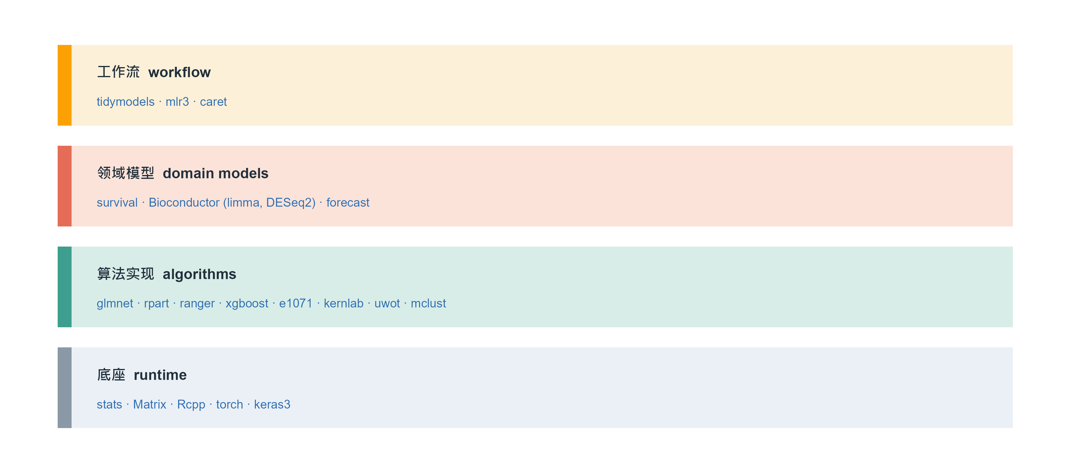
这十年这件事被补上了,而且补出了两套风格不同的方案。下图是现在 R 机器学习生态的分层:底下是算法实现,中间是统一接口,上面是工作流。
That gap has been closed over the last decade, in two quite different styles. The figure below layers the current R machine-learning stack: algorithms at the bottom, unified interfaces in the middle, workflows on top.
Figure 1: R 机器学习生态的四层。本文用到的包在第三层,工作流框架在第四层;第一层是几乎所有包都依赖的底座。分层不是为了排名,而是为了说明:同一个算法可以有三种调用方式,选哪一种取决于你要跑一个模型还是一百个。 | Four layers of the R machine-learning stack. The packages used here sit in layer 3, workflow frameworks in layer 4, and everything rests on layer 1. The layering is not a ranking: it shows that one algorithm can be called three ways, and which you choose depends on whether you need one model or a hundred.
A concrete comparison shows what the layering means in practice. The same job — five-fold cross-validated random forest on the Pima diabetes data — looks completely different in the three frameworks:
Code
# tidymodels: declare, then fit a workflowrf_spec <-rand_forest(trees =500) |>set_engine("ranger") |>set_mode("classification")rf_wf <-workflow() |>add_formula(type ~ .) |>add_model(rf_spec)rf_res <-fit_resamples(rf_wf, folds =vfold_cv(Pima.tr, v =5),metrics =metric_set(roc_auc, accuracy))collect_metrics(rf_res)
Code
# mlr3: build a task, a learner, then resampletask <-as_task_classif(Pima.tr, target ="type")learner <-lrn("classif.ranger", num.trees =500, predict_type ="prob")rr <-resample(task, learner, rsmp("cv", folds =5))rr$aggregate(msr("classif.auc"))
Code
# caret: one call, many modelsctrl <-trainControl(method ="cv", number =5,summaryFunction = twoClassSummary,classProbs =TRUE)train(type ~ ., data = Pima.tr, method ="ranger",trControl = ctrl, metric ="ROC")
All three do the same thing. The difference is style: tidymodels splits model and preprocessing into composable objects, which suits pipelines that must record every step; mlr3’s task/learner/measure triple suits running benchmarks over dozens of datasets; caret’s single train() call handles tuning and resampling together, which suits “I just need a working model now”. Section 7 completes this comparison.
1.1 本文的例子用什么数据 / What data the examples use
两套数据,一套通用一套生物学,避免”只有生物学家看得懂”和”举的例子和自己无关”这两种失败:
Two datasets, one general and one biological, to avoid both failure modes — examples nobody outside biology understands, and examples unrelated to the reader’s own work:
Pima 糖尿病数据(MASS::Pima.tr / Pima.te):200 个训练样本、332 个测试样本,7 个临床指标,预测是否为糖尿病。用来演示分类与集成方法。 Pima diabetes data (MASS::Pima.tr / Pima.te): 200 training and 332 test cases, seven clinical variables, predict diabetes. Used for classification and ensembles.
模拟表达矩阵:80 个样本 × 500 个基因,只有 8 个基因与结局真正相关。用来演示高维正则化与特征选择——这是生信里最典型的”p 远大于 n”场景,而且因为真值已知,可以验证方法有没有找回正确的基因。 A simulated expression matrix: 80 samples × 500 genes, of which 8 are truly associated. Used for high-dimensional penalisation and feature selection — the classic p ≫ n case in bioinformatics, and because the truth is known, we can check whether the method recovers the right genes.
The advantage of simulation is that you know the right answer. On real data you can only compare predictive error; on simulated data you can also ask whether the selected genes are the right ones — two different questions.
2. 一个视角看穿所有监督学习 / One lens for all supervised learning
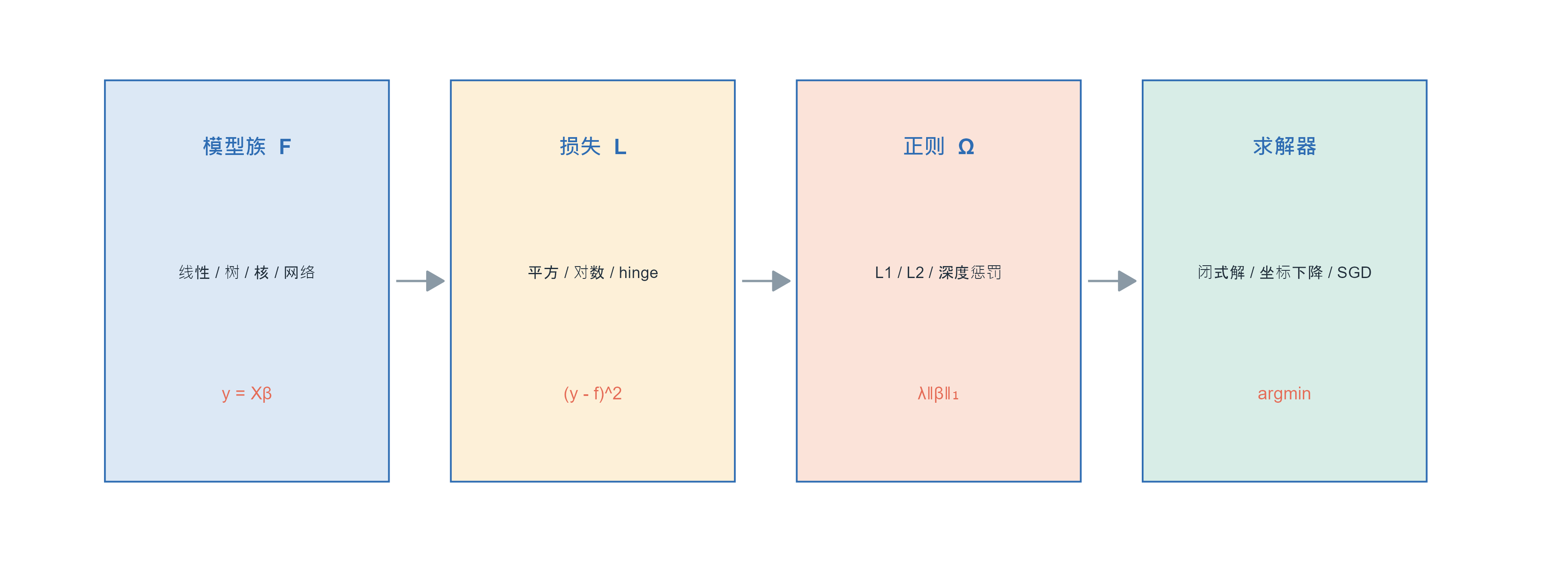
在写代码之前先建立这个视角,后面每一节都会回到它。几乎所有监督学习都在解同一个问题:
Build this lens before any code; every later section returns to it. Almost all supervised learning solves one problem:
\[\hat f=\arg\min_{f\in\mathcal{F}}\ \underbrace{\frac{1}{n}\sum_{i=1}^{n}L\big(y_i,f(x_i)\big)}_{\text{拟合数据 / fit the data}}+\ \underbrace{\lambda\,\Omega(f)}_{\text{别太复杂 / stay simple}}\]
Each term has a job: \(L\) says how wrong is wrong, \(\Omega\) says how complex is complex, and \(\lambda\) arbitrates. The set \(\mathcal{F}\) is the model family — linear functions, piecewise constants, sums of trees, the function class of a neural network.
Figure 2: 所有监督学习共用的一条流水线:模型族决定候选函数,损失函数决定怎么打分,正则项决定偏好哪一类解,优化算法负责把最小值找出来。换算法往往只是换了其中一格。 | Every supervised method shares one pipeline: the model family says which functions are candidates, the loss says how to score them, the penalty says which solutions to prefer, and the optimiser finds the minimum. Swapping algorithms usually swaps one cell.
把常见算法按这条流水线拆开,会看到它们其实很像:
Decompose the common algorithms along this pipeline and they look alike:
With this table, “algorithm” stops being mysterious: switching algorithms means switching one cell, and “tuning” is mostly tuning the third cell. In deep learning the only genuinely new thing is that \(\mathcal{F}\) becomes much larger; the other three cells are unchanged.
2.1 为什么需要正则:偏差与方差的真实形状 / Why regularise: the actual shape of bias and variance
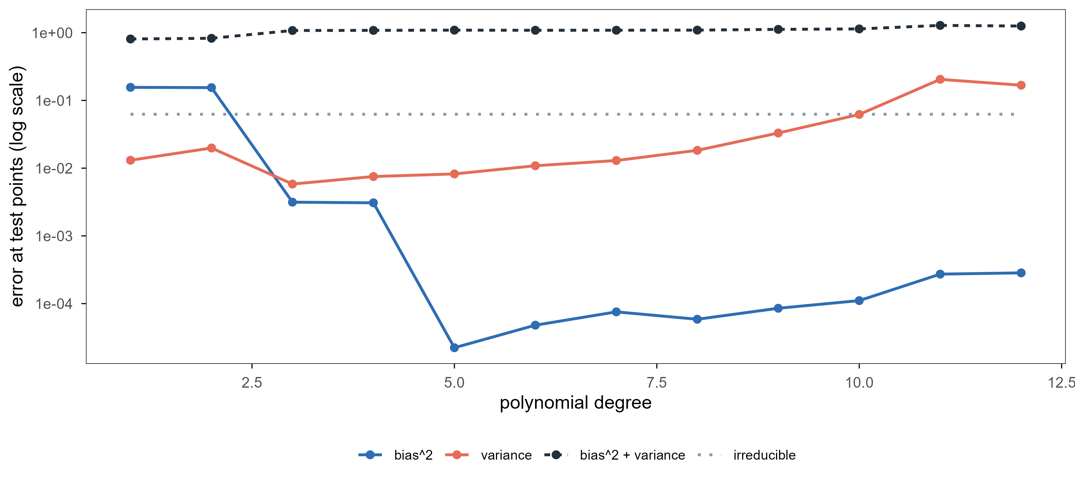
\(\Omega\) is not decoration. The simulation below computes the bias–variance trade-off instead of sketching it: fix the truth \(f(x)=\sin(2\pi x)\), fit polynomials of increasing degree, repeat the sampling 300 times, and estimate squared bias and variance at the test points.
Code
truth <-function(x) sin(2* pi * x)xgrid <-seq(0.05, 0.95, length.out =40)deg <-1:12R <-300noise <-0.25bias2 <-numeric(length(deg)); vari <-numeric(length(deg)); mse <-numeric(length(deg))for (k inseq_along(deg)) { preds <-matrix(NA_real_, R, length(xgrid))for (r inseq_len(R)) { x <-runif(45) y <-truth(x) +rnorm(45, 0, noise) fit <-lm(y ~poly(x, deg[k], raw =TRUE)) preds[r, ] <-predict(fit, newdata =data.frame(x = xgrid)) } m <-colMeans(preds) bias2[k] <-mean((m -truth(xgrid))^2) vari[k] <-mean(apply(preds, 2, var)) mse[k] <-mean(apply(preds, 2, function(v) mean((v -truth(xgrid))^2)))}bv <-rbind(data.frame(deg = deg, value = bias2, term ="bias^2"),data.frame(deg = deg, value = vari, term ="variance"),data.frame(deg = deg, value = mse, term ="bias^2 + variance"),data.frame(deg = deg, value =rep(noise^2, length(deg)), term ="irreducible"))bv$term <-factor(bv$term, levels =c("bias^2", "variance", "bias^2 + variance", "irreducible"))ggplot(bv, aes(deg, value, colour = term, linetype = term)) +geom_line(linewidth =0.8) +geom_point(data =subset(bv, term !="irreducible"), size =1.8) +scale_colour_manual(values =c("bias^2"= ml_pal[["blue"]], "variance"= ml_pal[["coral"]],"bias^2 + variance"= ml_pal[["ink"]],"irreducible"= ml_pal[["grey"]]), name =NULL) +scale_linetype_manual(values =c("bias^2"="solid", "variance"="solid","bias^2 + variance"="22", "irreducible"="dotted"),name =NULL) +scale_y_log10() +labs(x ="polynomial degree", y ="error at test points (log scale)") +theme(legend.position ="bottom", legend.text =element_text(size =8))
Figure 3: 偏差-方差的真实分解。阶数从 1 增到 12:偏差平方单调下降(模型更灵活),方差单调上升(对训练集更敏感),两者相加在 4 阶附近最低。纵轴是对数刻度。 | A computed bias–variance decomposition. As the degree goes from 1 to 12, squared bias falls monotonically (more flexible) and variance rises monotonically (more sensitive to the training set); their sum is lowest near degree 4. The vertical axis is logarithmic.
Three things to keep. First, the dashed total has a clear minimum, not at either end — the quantitative version of “not too simple, not too complex”. Second, variance grows roughly exponentially with degree (note the log axis) while bias falls ever more slowly, so past the optimum the error rises faster than it fell. Third, the noise floor (dotted) is a floor no model crosses — it sets the difficulty ceiling of the problem itself.
Every later “hyperparameter” — polynomial degree, KNN’s \(k\), tree depth, the penalty \(\lambda\) — moves along the same axis: left adds bias and removes variance, right does the reverse. Tuning is finding the minimum of that curve, and there is essentially one way to find it: hold out data that never takes part in fitting.
3. 线性模型与正则化:从最小二乘到 LASSO / Linear models and penalisation
3.1 最小二乘的解,以及它什么时候会崩 / The least-squares solution, and when it collapses
线性模型假设 \(f(x)=x^\top\beta\),平方损失下目标函数是
A linear model assumes \(f(x)=x^\top\beta\); with squared loss the objective is
Differentiate with respect to \(\beta\), set to zero, and the normal equations \(X^\top X\beta=X^\top y\) give \(\hat\beta=(X^\top X)^{-1}X^\top y\). Elegant — but it needs \(X^\top X\) to be invertible: the \(p\) features must be linearly independent and \(n\ge p\).
Bioinformatics data almost never satisfies that. With 500 genes and 80 samples, \(X^\top X\) is 500×500 but has rank at most 80, so it has infinitely many null directions; the solution is not unique, and the textbook one spreads weight over all genes with unusable variance. This is not a numerical nuisance — the problem has no unique answer. The penalty starts exactly here: among infinitely many equally good fits, pick one.
3.2 岭回归:给解加一条最小范数的偏好 / Ridge: prefer the smallest norm
Adding \(\lambda I\) makes the matrix invertible, which is why it is numerically stable. Statistically it shrinks: every coefficient is pulled toward zero proportionally, but never exactly to zero. As \(\lambda\to0\) it returns to least squares; as \(\lambda\to\infty\) everything goes to zero.
3.3 LASSO:让没用的变量变成精确的零 / LASSO: useless variables become exact zeros
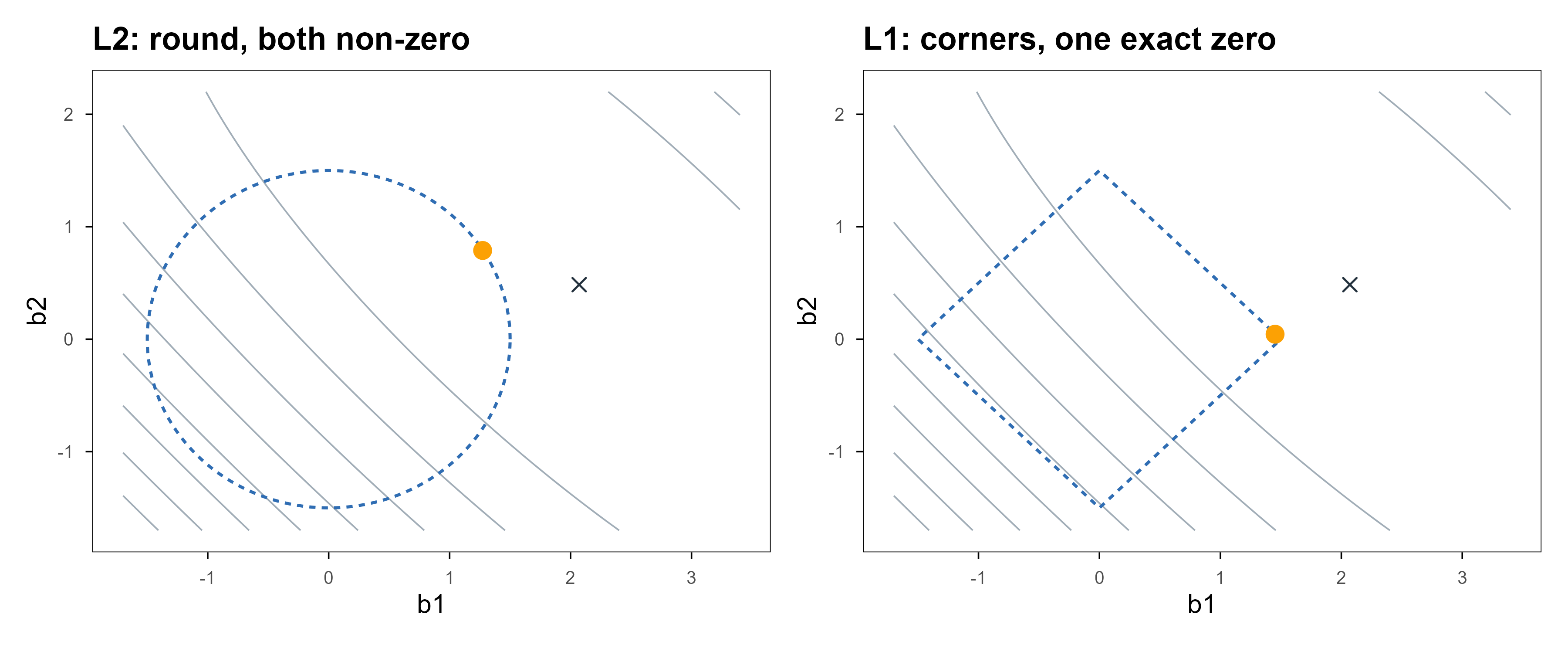
Swapping \(L_2\) for \(L_1\) changes the solution completely: \(\hat\beta\) becomes sparse, with many components exactly zero. The reason is geometric — the \(L_1\) ball has corners on the axes, and an expanding elliptical loss contour usually touches a corner first.
Figure 4: 两种约束的几何。灰色同心椭圆是残差平方和的等高线,虚线是可行域边界,橙点是数值上找到的最优解,叉号是最小二乘解。左:\(L_2\) 球是圆的,切点一般不在坐标轴上,两个系数都非零。右:\(L_1\) 球是菱形,切点落在角上,于是有一个系数恰好为 0。这就是 LASSO 稀疏的全部来源。 | Geometry of the two constraints. Grey contours are residual sum of squares, the dashed outline is the feasible region, the orange dot the numerically located optimum and the cross the least-squares solution. Left: the \(L_2\) ball is round, the contact is generically off-axis and both coefficients are non-zero. Right: the \(L_1\) ball is a diamond, the contact lands on a corner, so one coefficient is exactly zero. That is the whole origin of LASSO sparsity.
The cross is the least-squares solution (about \((2.20,0.40)\)) and the orange dot the constrained optimum. In the left panel both coefficients shrink but neither vanishes; in the right the second coefficient is pinned to an axis — that is where variable selection comes from. Not mysticism: the derivative of \(|\beta_j|\)jumps at zero, so no smooth direction can push the loss off that point once the constraint is tight enough.
Real solvers do not use a grid. glmnet uses coordinate descent: optimise one coefficient at a time with the rest fixed, which has a closed form (soft thresholding), sweep repeatedly, and it converges in a dozen passes. Because each subproblem is cheap and warm-starts from the previous solution, the whole \(\lambda\) path from large to small is often faster than one least-squares fit.
3.4 正则路径:把 λ 从大到小走一遍 / The regularisation path
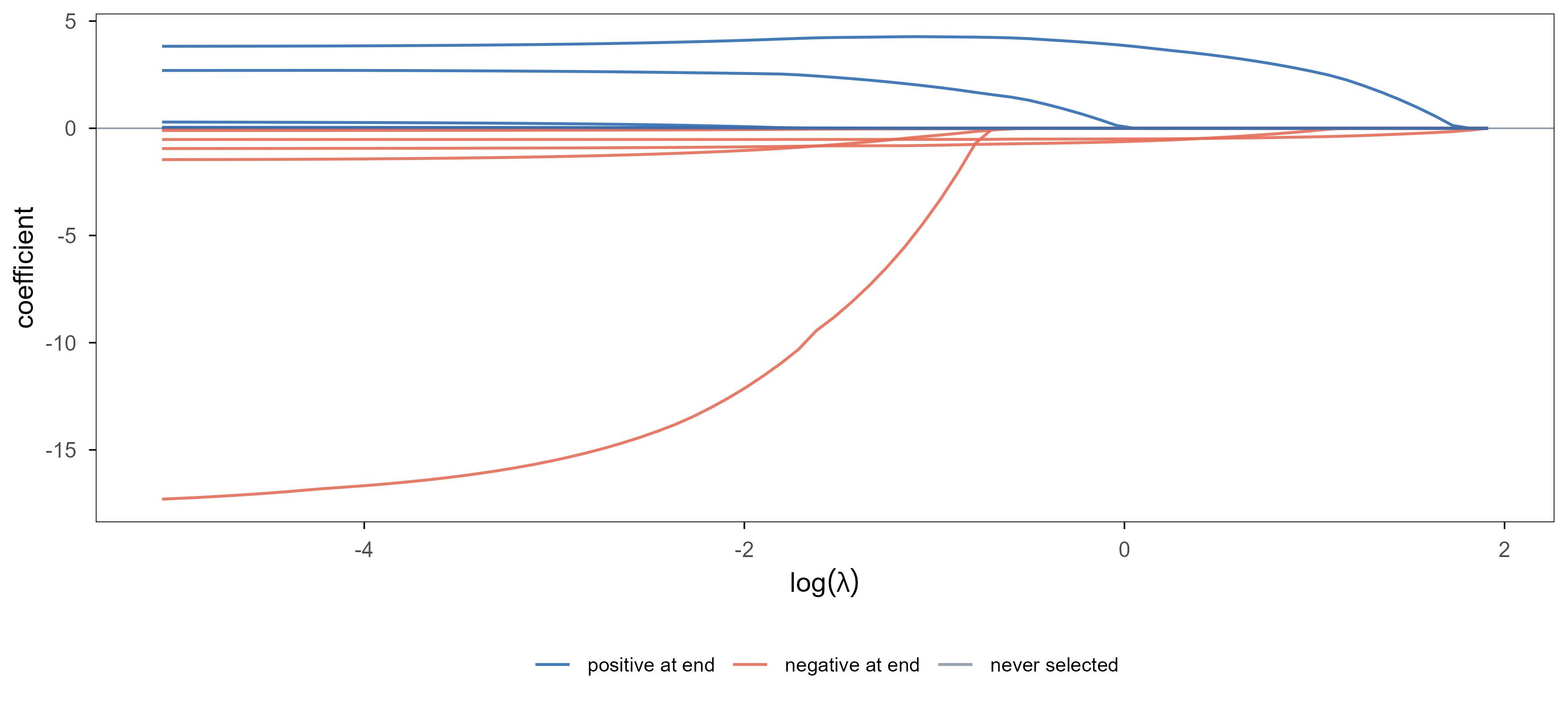
把 \(\lambda\) 当作自变量,画出每个系数随它的变化,能一眼看出”哪些变量先进入模型”。
Plot each coefficient against \(\lambda\) and you see at a glance which variables enter the model first.
Code
data(BostonHousing, package ="mlbench")bh <- BostonHousingXb <-model.matrix(medv ~ ., data = bh)[, -1]yb <- bh$medvfit_path <- glmnet::glmnet(Xb, yb, alpha =1)B <-as.matrix(fit_path$beta)path <-data.frame(loglam =rep(log(fit_path$lambda), each =nrow(B)),var =rep(rownames(B), times =ncol(B)),coef =as.vector(B))final <- B[, ncol(B)]path$grp <-ifelse(abs(final[path$var]) ==0, "never selected",ifelse(final[path$var] >0, "positive at end", "negative at end"))path$grp <-factor(path$grp,levels =c("positive at end", "negative at end", "never selected"))ggplot(path, aes(loglam, coef, group = var, colour = grp)) +geom_hline(yintercept =0, colour = ml_pal[["grey"]], linewidth =0.3) +geom_line(linewidth =0.55, alpha =0.9) +scale_colour_manual(values =c("positive at end"= ml_pal[["blue"]],"negative at end"= ml_pal[["coral"]],"never selected"= ml_pal[["grey"]]), name =NULL) +labs(x =expression(log(lambda)), y ="coefficient") +theme(legend.position ="bottom", legend.text =element_text(size =8))
Figure 5: 波士顿房价数据上的 LASSO 路径。横轴是 \(\log\lambda\),从左往右正则越来越强;每条曲线是一个预测变量。右端所有系数归零,说明正则足够强时模型退化成只预测均值。落在零线上的灰线是全程都没被选中的变量。 | LASSO path on the Boston housing data. The horizontal axis is \(\log\lambda\), increasing left to right; each curve is one predictor. At the right every coefficient is zero, so a strong enough penalty reduces the model to predicting the mean. Grey lines lying on zero are variables never selected.
Read it at three levels. First, everything is zero at the right end. Second, each curve leaves zero at a different point: variables leaving further right survive stronger penalties and are usually more important. Third, the curves push against each other — LASSO tends to keep only one of a highly correlated pair, and a different sample may keep the other. That instability is the direct reason the elastic net exists.
3.5 弹性网:两个惩罚项一起用 / Elastic net: both penalties at once
\(\alpha=1\) is LASSO and \(\alpha=0\) is ridge. Intermediate values both select variables and let correlated ones enter together. In bioinformatics this is nearly the default: genes are correlated within pathways, and pure LASSO picks one at random from each group, which reads badly.
3.6 高维案例:从 500 个基因里找回 8 个 / A p ≫ n case: recovering 8 genes out of 500
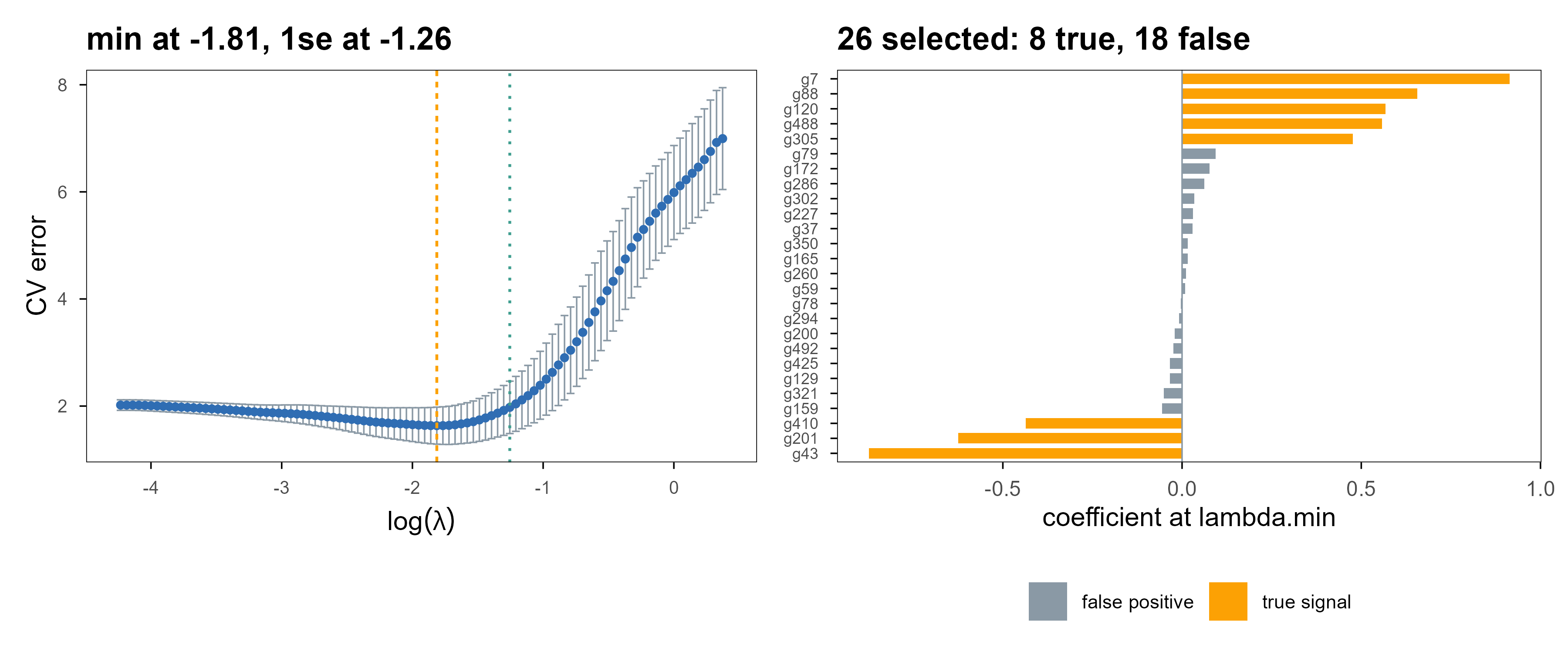
现在做那个真正的问题:80 个样本、500 个基因,只有 8 个基因与结局相关,其余是纯噪声。
Now the real question: 80 samples, 500 genes, only 8 associated with the outcome, the rest pure noise.
Figure 6: 高维情形下的交叉验证与变量选择。左:五折交叉验证曲线,虚线是最优 \(\lambda\)。右:该 \(\lambda\) 下系数非零的基因,橙色是真正有效的 8 个,灰色是被误选的。稀疏方法在相关设计下的典型表现是找回大部分真信号、同时带进少量假阳性。 | Cross-validation and selection in the p ≫ n case. Left: the five-fold CV curve with the optimal \(\lambda\) marked. Right: genes with non-zero coefficients at that \(\lambda\); orange are the 8 truly associated, grey are false positives. Sparse methods under correlated designs typically recover most of the signal and admit a few false positives.
The result: at \(\lambda_{\min}\), 26 genes are selected — 8 true, 18 false positives, 0 missed. Switching to the one-standard-error rule (\(\lambda_{1se}\), the dotted line) shrinks the set to 12 genes, still containing 8 of the true ones. Those numbers set up the three points below.
First, false positives are not a bug. LASSO’s guarantee is about prediction error (near-optimal when \(\lambda\) is chosen well), not “the selected set equals the true set”. The latter needs stronger conditions and dedicated machinery (stability selection, knockoffs). Second, how you pick \(\lambda\) decides the conclusion: lambda.min optimises prediction error and therefore keeps more variables; lambda.1se picks the simplest model within one standard error of the minimum, which is usually smaller and more stable. Both are right — it depends on whether you want prediction or explanation. Third, and most important, real data give you no ground truth — so report whether the selected genes enrich for known pathways instead of claiming to have found “the right” ones.
The package mapping: lm() and glm() are the unpenalised baselines; glmnet covers ridge, LASSO, elastic net and their generalised-linear versions (family = "binomial" gives penalised logistic regression); ncvreg and grpreg handle non-convex penalties and group structure. In daily work glmnet alone is enough.
4. 分类:从概率到边界 / Classification: from probabilities to boundaries
Classification predicts a probability or a label, not a number. This section groups methods by how they define the boundary: logistic regression gives a linear boundary, KNN a local one, and SVM a maximum-margin one. Three inductive biases, none universally better.
4.1 逻辑回归:把线性输出压成概率 / Logistic regression: squashing a linear output into a probability
This loss is the log-loss, or cross-entropy. Why not squared error? Because \(\sigma\) is nearly flat for large \(|z|\), so the gradient of a squared loss with respect to \(z\) vanishes — the model learns slowest exactly when it is most wrong. Log-loss has gradient \((\sigma(z)-y)\) with respect to \(z\): the further off, the larger the push.
The solver is iteratively reweighted least squares, i.e. Newton’s method; one glm() call does it. The coefficients read directly: \(e^{\beta_j}\) is the odds ratio for a one-unit increase in \(x_j\). For a clinical audience that beats “feature importance” — it gives a direction and a multiplier.
The boundary is \(w^\top x+b=0\), a hyperplane. So it can only express linearly separable structure; for a curved boundary you either add interactions and splines by hand, or change method.
4.2 KNN:不训练,只查邻居 / KNN: no training, just neighbours
KNN 把训练集原样存下来。预测新样本时,找距离最近的 \(k\) 个训练点,多数票决定类别:
KNN stores the training set as-is. To predict, find the \(k\) nearest training points and take a majority vote:
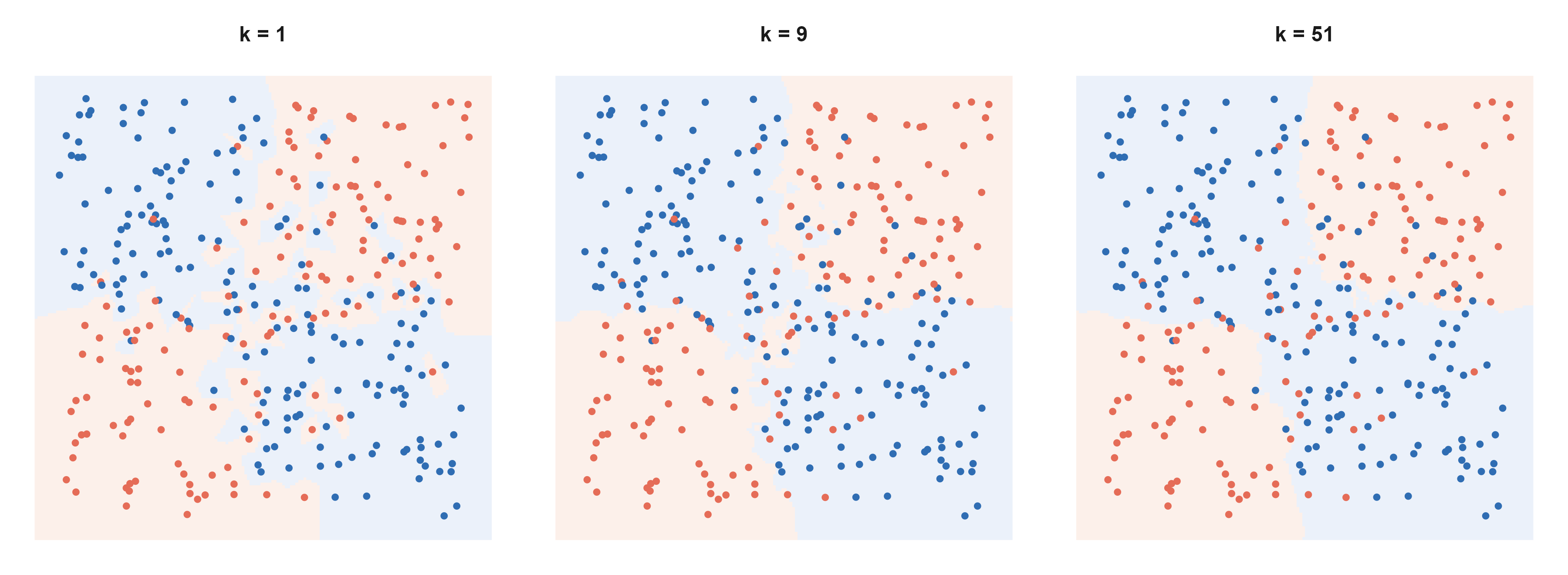
It estimates the local frequency of \(P(y=1\mid x)\) near \(x\), so larger \(k\) means smoother and more biased; at \(k=1\) the training error is exactly zero while the boundary jitters with every sample.
Figure 7: 同一个数据集、同一个距离度量,只改 \(k\)。真实规律是「两个变量同号 vs 异号」的四象限结构,并带有标签噪声。\(k=1\) 时边界被单个噪声点拉扯,出现碎片与孤岛;\(k=9\) 时已经接近真实的四象限;\(k=51\) 时过度平滑,象限结构只剩下粗略的东西分界。三张图用的是同一份训练数据。 | Same data, same distance, only \(k\) changes. The true rule is a four-quadrant pattern (same sign versus opposite signs of the two variables) with label noise. At \(k=1\) the boundary is dragged by individual noisy points and fragments into islands; at \(k=9\) it approaches the true quadrants; at \(k=51\) it is over-smoothed and only a crude left-right split survives. All three use the same training data.
Two limits must be known. First, standardise first: otherwise the variable with the largest scale owns the distance. Second, high dimensions break it: as dimension grows, the ratio of nearest to farthest distance approaches 1, so the “nearest” neighbour stops being near — the curse of dimensionality. With 500 genes all distances look alike, which is why KNN usually does badly on expression data; it suits low-dimensional problems with irregular boundaries.
4.3 SVM:把边界推到最宽 / SVM: push the boundary as far as it goes
同样找线性边界,SVM 加了一条要求:边界到两类最近点之间的间隔要最大。写成优化问题是
SVM also seeks a linear boundary, with one extra requirement: maximise the margin between the boundary and the nearest points of each class. As an optimisation problem:
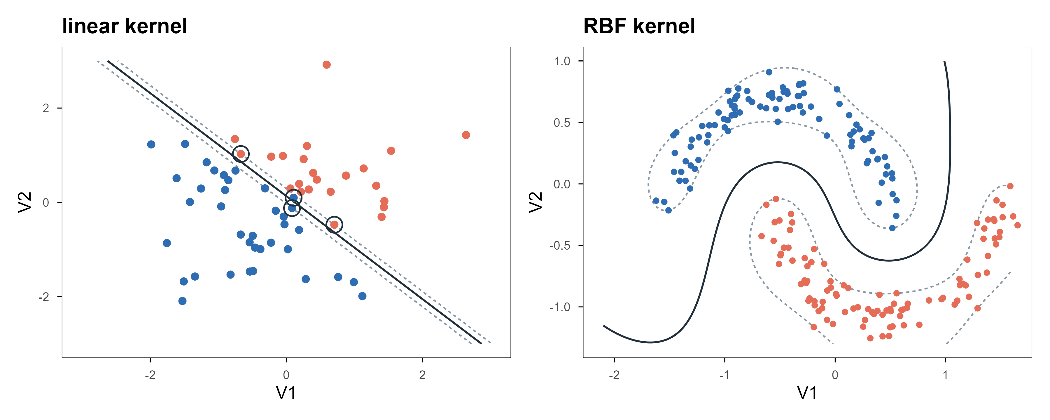
约束里取等号的点就是支持向量,边界完全由它们决定,其余样本删掉结果不变——这是 SVM 与逻辑回归最本质的差别:它只看”最难分的那些点”。允许少量越界时把约束放松,等价于用 hinge 损失 \(\max(0,1-y f(x))\) 代替 log-loss 做正则化经验风险最小化。
The points where the constraint is tight are the support vectors; the boundary is determined entirely by them, and deleting the other samples changes nothing. That is the essential difference from logistic regression: it looks only at the hardest points. Allowing some violations relaxes the constraint and is equivalent to using the hinge loss \(\max(0,1-y f(x))\) inside regularised empirical risk minimisation.
Figure 8: 左:线性核的间隔。实线是决策边界,两条虚线是间隔边界(决策值 \(\pm1\)),圈出的点是支持向量——把其他点全删掉,边界不变。右:换成 RBF 核之后,同一个算法在两个交错的半月形上给出弯曲边界,而不需要手工造特征。 | Left: a linear-kernel margin. The solid line is the boundary, the dashed lines are the margin edges (decision value \(\pm1\)), and the circled points are support vectors — delete every other point and the boundary does not move. Right: with an RBF kernel the same algorithm produces a curved boundary on two interleaved moons, with no hand-built features.
The right panel is possible because of the kernel trick: replace the inner product \(x_i^\top x_j\) with a kernel \(k(x_i,x_j)\), which is equivalent to mapping into a higher-dimensional space and separating there, without ever computing the map. The RBF kernel \(k(x,x')=\exp(-\gamma\|x-x'\|^2)\) corresponds to an infinite-dimensional feature space. The price is an \(n\times n\) kernel matrix, which on large samples costs both memory and time — one reason SVMs lost ground to tree ensembles as datasets grew.
In practice e1071::svm is the usual interface (classification, regression, one-class), wrapping libsvm; kernlab offers a more R-idiomatic formula interface and more kernels; for large samples with a linear kernel, LiblineaR is faster. Tuning is mostly two numbers: cost controls how many violations are tolerated, gamma controls how curved the boundary gets.
4.4 判别分析:一类被低估的线性方法 / Discriminant analysis: an underrated linear method
MASS::lda() takes another route: assume each class is multivariate normal with a shared covariance, then invert Bayes to get the posterior. Mathematically the resulting boundary is nearly the same linear one as logistic regression; the difference is how it is estimated. Logistic regression is discriminative (fit \(P(y\mid x)\) directly), LDA is generative (fit \(P(x\mid y)\) and invert). When classes are well separated, samples are few, or \(p\) approaches \(n\), the generative assumption can be more data-efficient; when normality clearly fails, logistic regression is safer. qda() drops the shared covariance and yields a quadratic boundary with more parameters.
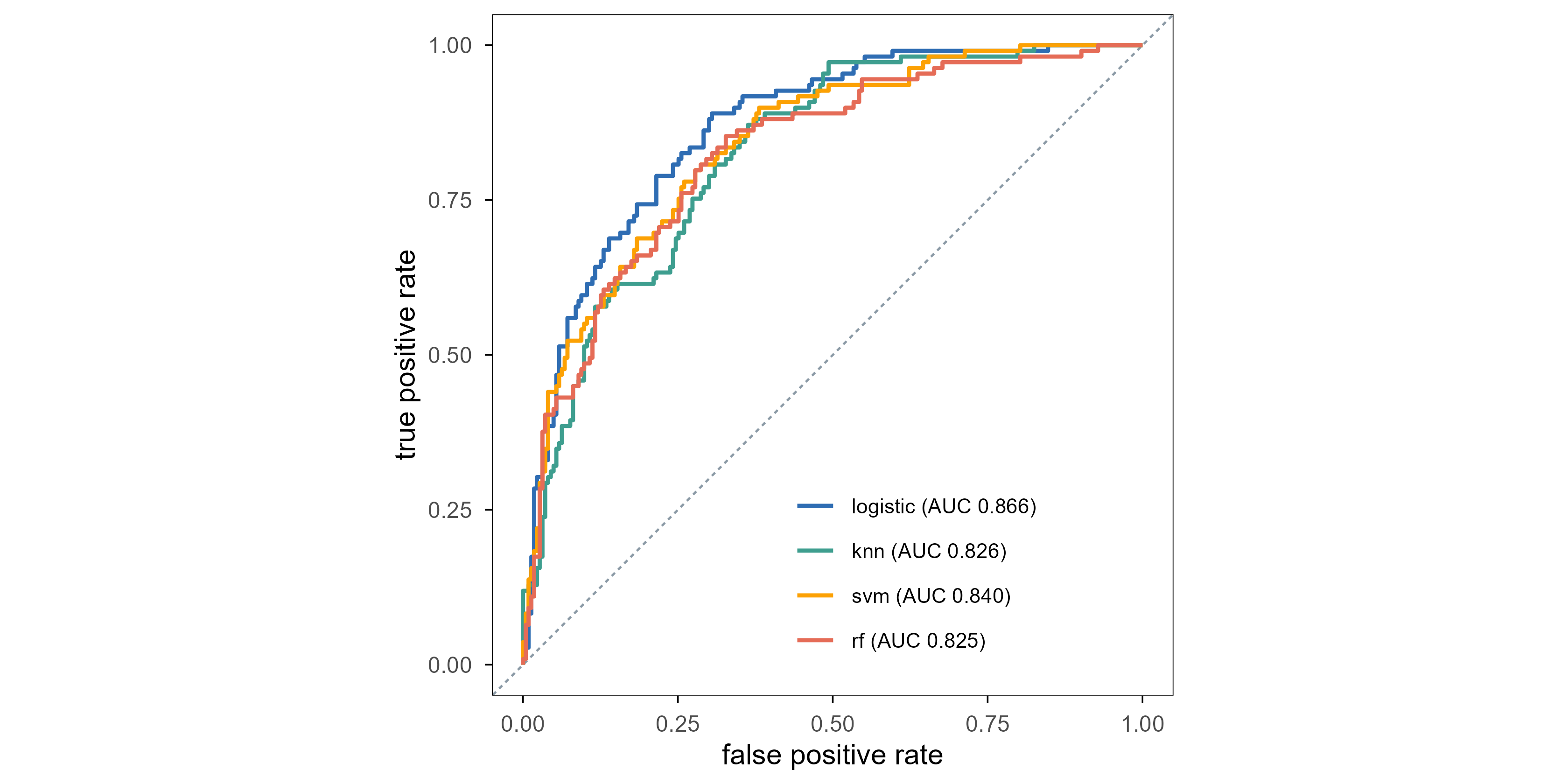
Enough theory; look at numbers. Fit four models on the 200 Pima training cases and evaluate ROC and AUC on the 332 held-out cases. Every preprocessing parameter is estimated on the training set only — section 7 returns to why.
Figure 9: 四个模型在同一个测试集上的 ROC。对角线是随机猜测。最朴素的逻辑回归反而最高(AUC 0.866),三个更复杂的模型都落在 0.83 附近,彼此相差不到 0.02。在 332 个测试样本上,这个量级的差别与置信区间同阶——它说明的是「复杂度没有换来提升」,而不是「逻辑回归更好」。 | ROC for four models on the same test set. The diagonal is chance. The plainest model, logistic regression, comes out highest (AUC 0.866); the three more complex ones sit near 0.83, within 0.02 of each other. On 332 test cases a difference of this size is the same order as the confidence interval — the figure says that complexity bought nothing, not that logistic regression is better.
The AUCs are 0.866 (logistic regression), 0.826 (KNN), 0.840 (SVM) and 0.825 (random forest). The result is mildly counter-intuitive: the plainest model wins. The three complex ones cluster near 0.83 within 0.02 of each other, while logistic regression is about 0.04 ahead.
Before concluding, do the arithmetic: with 332 test cases and about a third of them positive, the standard error of an AUC is roughly 0.02–0.03. So the gap between 0.866 and 0.840 is “possible”, not “established”; what the data do support is the weaker statement: on this problem, complexity brought no gain.
This is not “random forests are bad” but that model complexity must match the information in the data. The same forest on 500 genes and 800 samples, or on a table with strong interactions, will lead clearly. So when you read “model X has higher AUC”, the first question is always: on what data, at what sample size, and is the gap larger than the confidence interval.
5. 树与集成:分段常数为什么这么能打 / Trees and ensembles
5.1 CART:递归地把空间切成方块 / CART: recursively cut the space into boxes
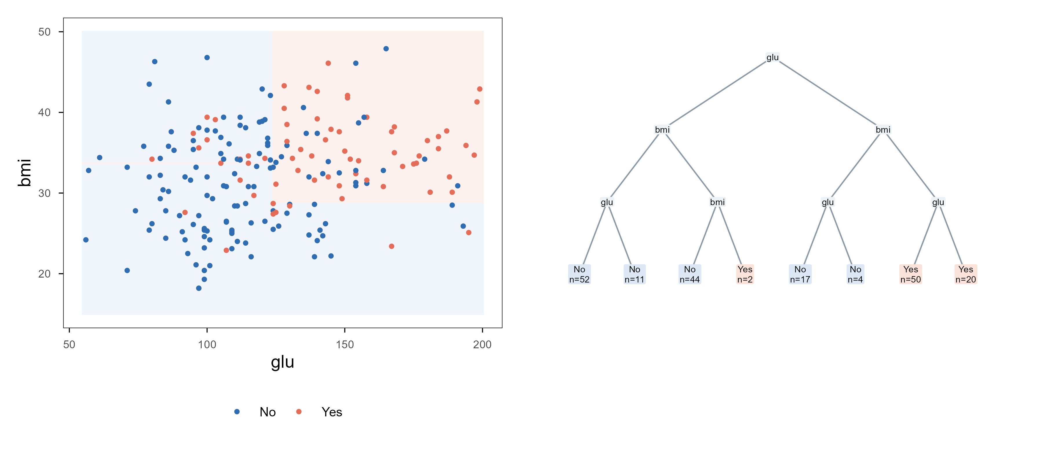
A decision tree assumes \(f\) is piecewise constant: cut the feature space into boxes and assign one constant per box. The cutting is recursive — at each step choose one variable and one threshold, and split the current region in two.
切在哪里的判据是”不纯度下降最多”。分类问题常用 Gini 指数
The criterion is the largest drop in impurity. For classification the usual choice is the Gini index
Regression trees use the reduction in squared error. Both are greedy: each step takes the locally best split with no backtracking. Greedy is why trees are cheap (roughly \(O(np\log n)\)) and why they are unstable — move a few points and the whole tree can change.
Figure 10: 左:一棵深度 3 的树在 (glu, bmi) 平面上划出的区域,颜色是预测类别,点是训练样本。右:同一棵树的结构,内部节点标出用来分裂的变量,叶子给出类别与该叶子的样本数。分段常数的边界一定是横平竖直的矩形——这是树能表达什么、不能表达什么的根源。 | Left: the regions a depth-3 tree carves out in the (glu, bmi) plane, coloured by predicted class, with training points on top. Right: the same tree; internal nodes show the splitting variable, leaves show the class and the number of cases. Piecewise-constant boundaries are always axis-aligned rectangles — the root of what a tree can and cannot express.
The figure exposes the fundamental limit: boundaries can only be axis-aligned, so a diagonal boundary needs many small boxes to approximate. The benefits are scale invariance (changing units does not change the splits), automatic interactions (each root-to-leaf path is a conjunction of conditions), and robustness to outliers in a single feature. The cost is that one tree has enormous variance — which is what the next section fixes.
5.2 Bagging 与随机森林:用平均换方差 / Bagging and random forests: trading variance for an average
If one tree has high variance, the direct fix is to train many and average. Bagging draws \(B\) bootstrap samples of the training set, fits a deep tree on each, and averages at prediction time.
The second term vanishes as \(B\) grows; the first does not — which is why random forests exist. Adding trees alone leaves variance stuck at the correlation floor. A random forest draws only \(m\approx\sqrt p\) candidate variables at each split, deliberately lowering \(\rho\) so the first term shrinks too.
Code
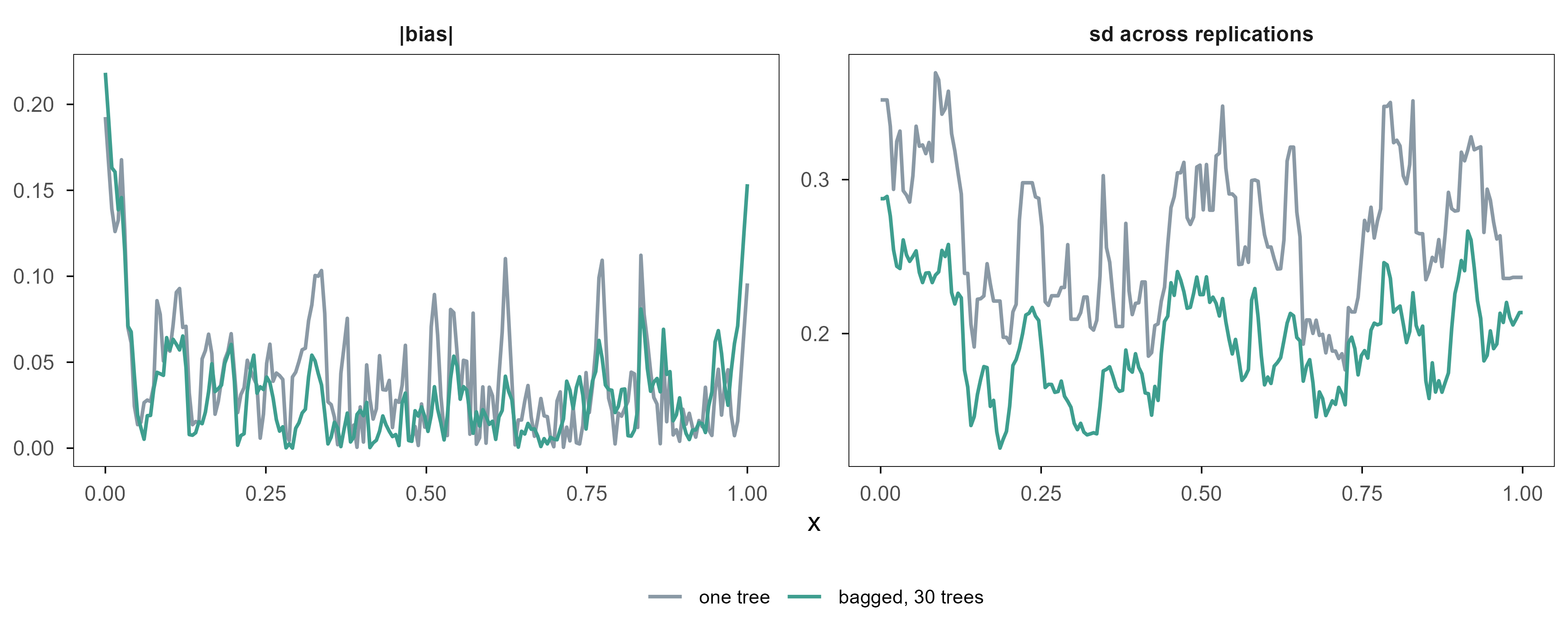
set.seed(20261101)true_f <-function(x) 0.8*sin(2* pi * x) +0.3* xxgrid <-seq(0, 1, length.out =200)n_tr <-60; R <-25; B <-30ctrl <- rpart::rpart.control(maxdepth =5, cp =0.001, minsplit =5)single <-matrix(NA_real_, R, length(xgrid))bagged <- singlefor (r inseq_len(R)) { x <-runif(n_tr); y <-true_f(x) +rnorm(n_tr, 0, 0.35) d <-data.frame(x = x, y = y) single[r, ] <-predict(rpart::rpart(y ~ x, data = d, control = ctrl),data.frame(x = xgrid)) boot <-matrix(NA_real_, B, length(xgrid))for (b inseq_len(B)) { db <- d[sample(n_tr, replace =TRUE), ] boot[b, ] <-predict(rpart::rpart(y ~ x, data = db, control = ctrl),data.frame(x = xgrid)) } bagged[r, ] <-colMeans(boot)}var_single <-mean(apply(single, 2, var))var_bag <-mean(apply(bagged, 2, var))pd <-rbind(data.frame(x = xgrid, v =sqrt(apply(single, 2, var)), model ="one tree",q ="sd across replications"),data.frame(x = xgrid, v =sqrt(apply(bagged, 2, var)), model ="bagged, 30 trees",q ="sd across replications"),data.frame(x = xgrid, v =abs(colMeans(single) -true_f(xgrid)), model ="one tree",q ="|bias|"),data.frame(x = xgrid, v =abs(colMeans(bagged) -true_f(xgrid)), model ="bagged, 30 trees",q ="|bias|"))pd$model <-factor(pd$model, levels =c("one tree", "bagged, 30 trees"))ggplot(pd, aes(x, v, colour = model)) +geom_line(linewidth =0.7) +facet_wrap(~ q, scales ="free_y") +scale_colour_manual(values =c("one tree"= ml_pal[["grey"]],"bagged, 30 trees"= ml_pal[["teal"]]), name =NULL) +labs(x ="x", y =NULL) +theme(legend.position ="bottom", legend.text =element_text(size =8))
Figure 11: 重复 25 次独立抽样,在 200 个测试点上分别估计两件事。左:预测的标准差(方差的平方根),单棵树明显更抖,平均 30 棵之后降到约七成。右:偏差的绝对值,两条曲线几乎重合——平均没有改变偏差。纵轴各自独立,因为要看的是同侧两条曲线的相对位置。 | Twenty-five independent samples, with two quantities estimated at 200 test points. Left: the standard deviation of the prediction; a single tree is visibly noisier and averaging 30 trees cuts it to about seventy percent. Right: absolute bias, where the two curves nearly coincide — averaging does not change bias. The vertical axes are independent because the comparison of interest is between the two curves within each panel.
On the same test grid the prediction variance of a single tree is 0.072; averaging 30 trees reduces it to 0.040, i.e. 55% of the original, while the two bias curves virtually overlap. Averaging touches variance, not bias, exactly as the bias–variance decomposition says.
Note the drop is only around half, and adding more trees will not push it further. That is the \(\rho\sigma^2\) term talking: trees grown on the same training data are highly correlated, and \(\rho\) does not shrink as \(B\) grows. The mtry knob in a random forest exists precisely to lower \(\rho\) — each tree sees a random subset of variables, so the trees genuinely disagree.
That also means bagging cannot rescue a badly biased model. If each tree is too shallow (two cuts only), averaging a thousand of them gives the same two cuts. Random forests therefore use deep trees — low bias, high variance — and buy the variance back with averaging.
5.3 梯度提升:一再加一点点 / Gradient boosting: add a little, repeatedly
Boosting works the other way: instead of training many trees in parallel, it fits them in sequence, each one correcting the residual left by all previous trees.
\(\eta\) is the learning rate (shrinkage). Each \(h_m\) is usually a very shallow tree (depth 1–3) because it only has to fit “what is left”. This is gradient boosting: the residual is the negative gradient under squared loss, and swapping the loss (to logistic, say) turns “fit the residual” into “fit the negative gradient” with the same structure.
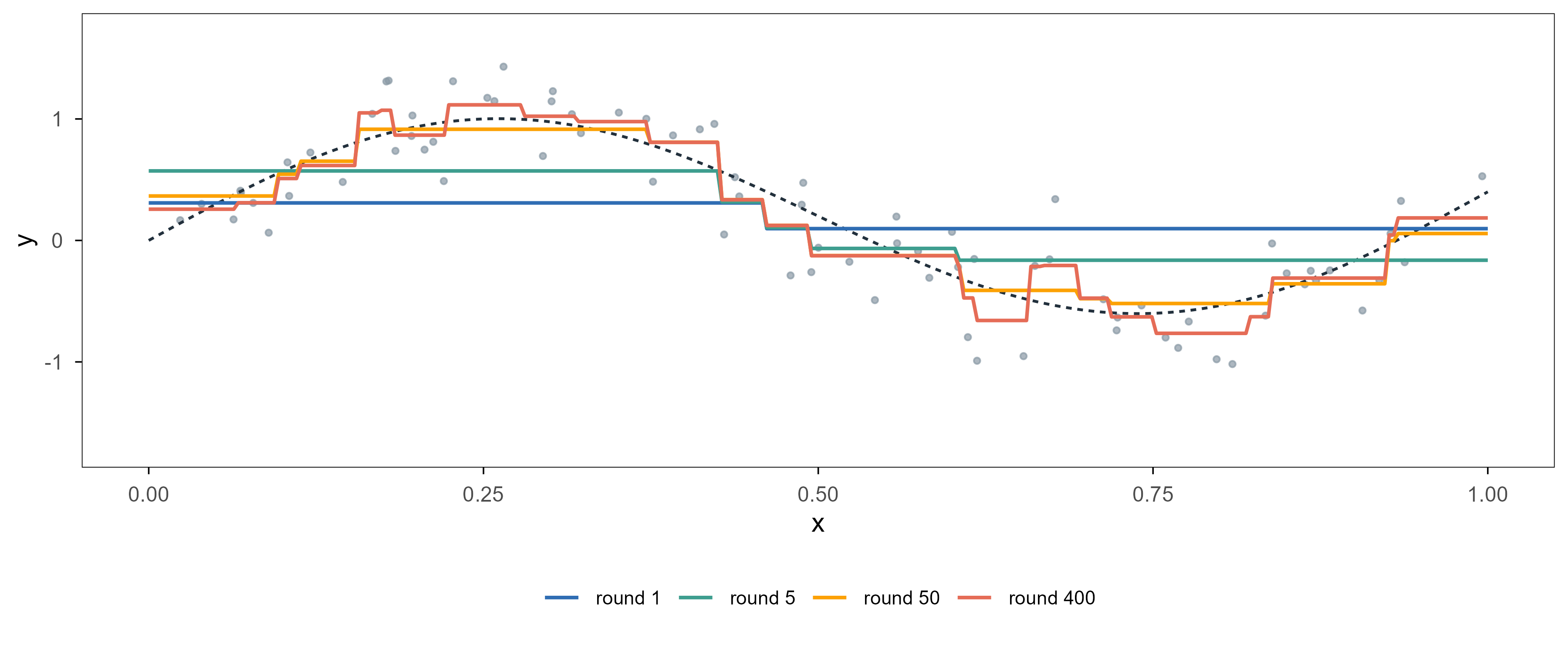
Code
set.seed(20261101)gb_true <-function(x) 0.9*sin(2* pi * x) +0.4* xx <-sort(runif(80))y <-gb_true(x) +rnorm(80, 0, 0.3)xgr <-data.frame(x =seq(0, 1, length.out =300))ctrl1 <- rpart::rpart.control(maxdepth =1, cp =0, minsplit =5)eta <-0.2; M <-400g <-rep(mean(y), nrow(xgr))f <-rep(mean(y), length(x))store <-list()for (m inseq_len(M)) { r <- y - f h <- rpart::rpart(r ~ x, data =data.frame(x = x, r = r), control = ctrl1) f <- f + eta *predict(h, data.frame(x = x)) g <- g + eta *predict(h, xgr)if (m %in%c(1, 5, 50, 400)) { store[[as.character(m)]] <-data.frame(x = xgr$x, y = g, stage =paste0("round ", m)) }}gbdf <-do.call(rbind, store)gbdf$stage <-factor(gbdf$stage,levels =c("round 1", "round 5", "round 50", "round 400"))ggplot(gbdf, aes(x, y, colour = stage)) +geom_point(data =data.frame(x = x, y = y), aes(x, y), inherit.aes =FALSE,colour = ml_pal[["grey"]], size =0.9, alpha =0.7) +geom_line(data =data.frame(x = xgr$x, y =gb_true(xgr$x)),aes(x, y), inherit.aes =FALSE,colour = ml_pal[["ink"]], linetype ="22", linewidth =0.55) +geom_line(linewidth =0.7) +scale_colour_manual(values =unname(ml_pal[c("blue", "teal", "orange", "coral")]),name =NULL) +coord_cartesian(ylim =c(-1.7, 1.7)) +labs(x ="x", y ="y") +theme(legend.position ="bottom", legend.text =element_text(size =8))
Figure 12: 梯度提升的逐步拟合。每一轮加一棵深度 1 的树,学习率 0.2。第 1 轮只能给出一个阶梯,第 5 轮已经抓住大致形状,第 50 轮贴住数据,第 400 轮开始把噪声也学了进去。树的数量在这里就是光滑度参数。 | Stagewise fitting in gradient boosting. One depth-1 tree is added per round with learning rate 0.2. After one round the fit is a single step; by round 5 it has the broad shape; by round 50 it tracks the data; by round 400 it starts fitting noise. The number of trees is a smoothness parameter here.
Compare this with the previous figure and the two ensembles move in opposite directions: bagging lets every tree overfit and cancels the variance by averaging; boosting keeps every tree weak and reduces bias by accumulation. So a forest tunes mtry (tree correlation) and depth, while boosting tunes the learning rate and the number of rounds — and needs early stopping, because the round-400 curve is already learning noise.
5.4 变量重要性与部分依赖:集成模型怎么解释 / Importance and partial dependence
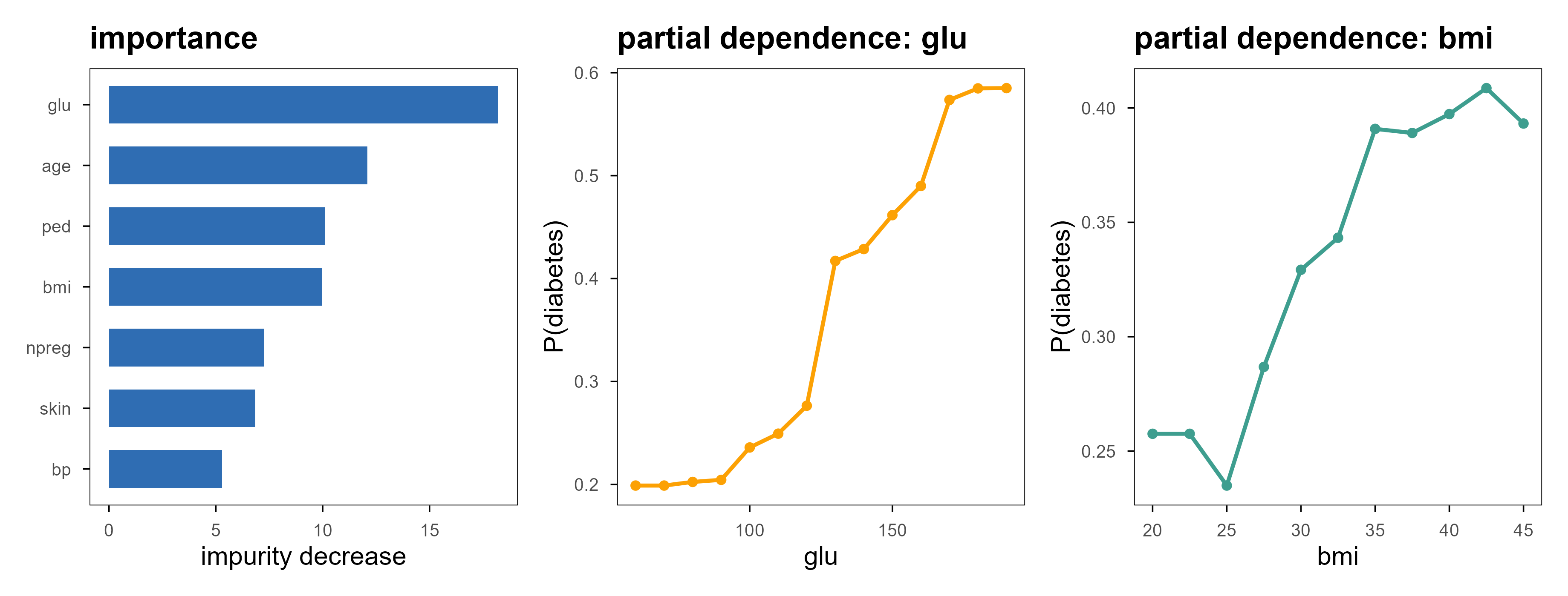
Forests and boosted models have no coefficients to read, but two tools still work. Variable importance sums the impurity decrease each variable contributes across all splits; a partial dependence plot forces one variable through a range of values while holding the others as they are, and tracks the average prediction.
Figure 13: 左:随机森林在不纯度意义下的变量重要性,血糖(glu)遥遥领先。中、右:glu 与 bmi 的部分依赖曲线,纵轴是预测为糖尿病的平均概率。注意 PDP 是平均效应,当变量与其他变量有强交互时,它可能掩盖掉个体层面的相反趋势。 | Left: impurity-based importance from a random forest; glucose (glu) leads by a wide margin. Middle and right: partial dependence for glu and bmi, with the vertical axis showing the average predicted probability of diabetes. Note that a PDP is an average effect; under strong interactions it can hide opposite trends at the individual level.
Impurity importance has a known bias: it favours variables with many distinct values. A continuous variable offers countless cut points, so a forest more easily finds a split that looks useful, and its score inflates. The more reliable option is permutation importance (importance = "permutation"): shuffle one variable and measure how much performance drops. It costs extra prediction passes but answers a question closer to “does this variable actually help predict”.
5.5 四个包的取舍 / Choosing among four packages
包 / Package
能做什么 / What it does
优点 / Strength
注意 / Caveat
rpart
单棵 CART,分类与回归
可解释、能画树、带代价矩阵
方差大,别单独用来预测
ranger
随机森林(C++ 后端)
快、支持 OOB 与 case weights、内存省
分类概率需校准
xgboost
梯度提升
正则化目标、早停、原生缺失值处理、SHAP
参数多,调参成本高
gbm
梯度提升(较老)
接口简单、支持分布族
慢,社区活跃度低
English
Package
What it does
Strength
Caveat
rpart
single CART tree, classification and regression
interpretable, plottable, cost matrices
high variance; do not use alone for prediction
ranger
random forest (C++ backend)
fast, out-of-bag estimates, case weights
probabilities need calibration
xgboost
gradient boosting
regularised objective, early stopping, native missing values, SHAP
On tabular data, xgboost or ranger is usually the first model to try: insensitive to feature scaling, automatic interactions, tolerant of missing values. They are also the easiest to misuse — not because the model is too strong, but because tuning and validation were not done properly (section 7).
6. 无监督:没有标签时在优化什么 / Unsupervised learning: what is optimised without labels
Without \(y\) there is no “predicted correctly”. Unsupervised methods can only optimise structure in the data itself: distances between points, tightness within clusters, directions of variance. Keep that in mind and you will not expect a “correct answer”.
6.1 K-means:最小化簇内平方和 / K-means: minimise within-cluster sum of squares
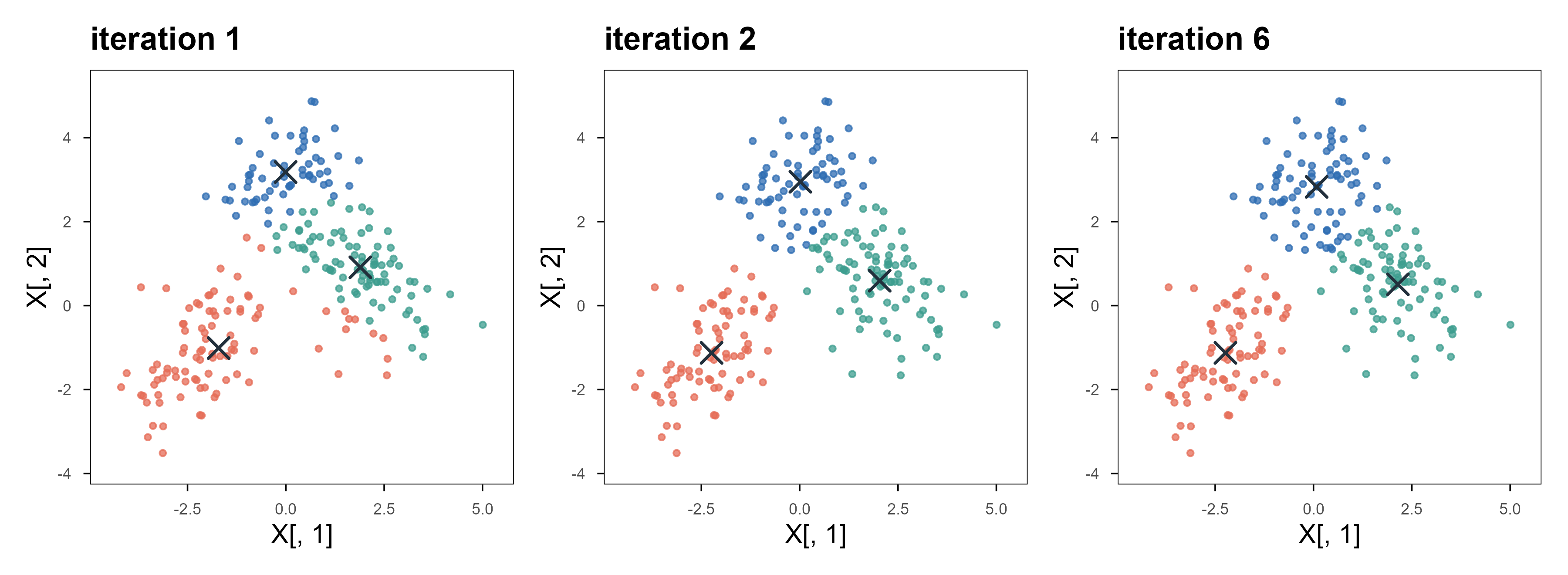
The solver is Lloyd’s algorithm, alternating two steps: assign each point to the nearest centre, then update each centre to the mean of its members. Both steps decrease the objective, so it always converges — but only to a local optimum, which depends on the initialisation. That is why nstart exists.
Figure 14: K-means 的三次迭代。灰叉是当前的中心,颜色是当前的分配。第 1 次迭代的边界还很粗糙,到第 6 次已经稳定。注意边界始终是直线段——这来自欧氏距离的几何,不是数据本身的性质。 | Three iterations of K-means. Grey crosses are the current centres, colours the current assignment. After one iteration the boundary is still crude; by iteration 6 it is stable. Note the boundaries are always straight segments — that comes from Euclidean geometry, not from the data.
Three limits must be known. First, you supply \(K\); the algorithm will not tell you how many clusters there are. Second, it implicitly assumes spherical, similar-sized clusters: two elongated, interleaved clusters get cut down the middle. Third, it is scale-sensitive — standardise first.
6.2 层次聚类:先造一棵树,再决定切几刀 / Hierarchical clustering: build a tree, then cut it
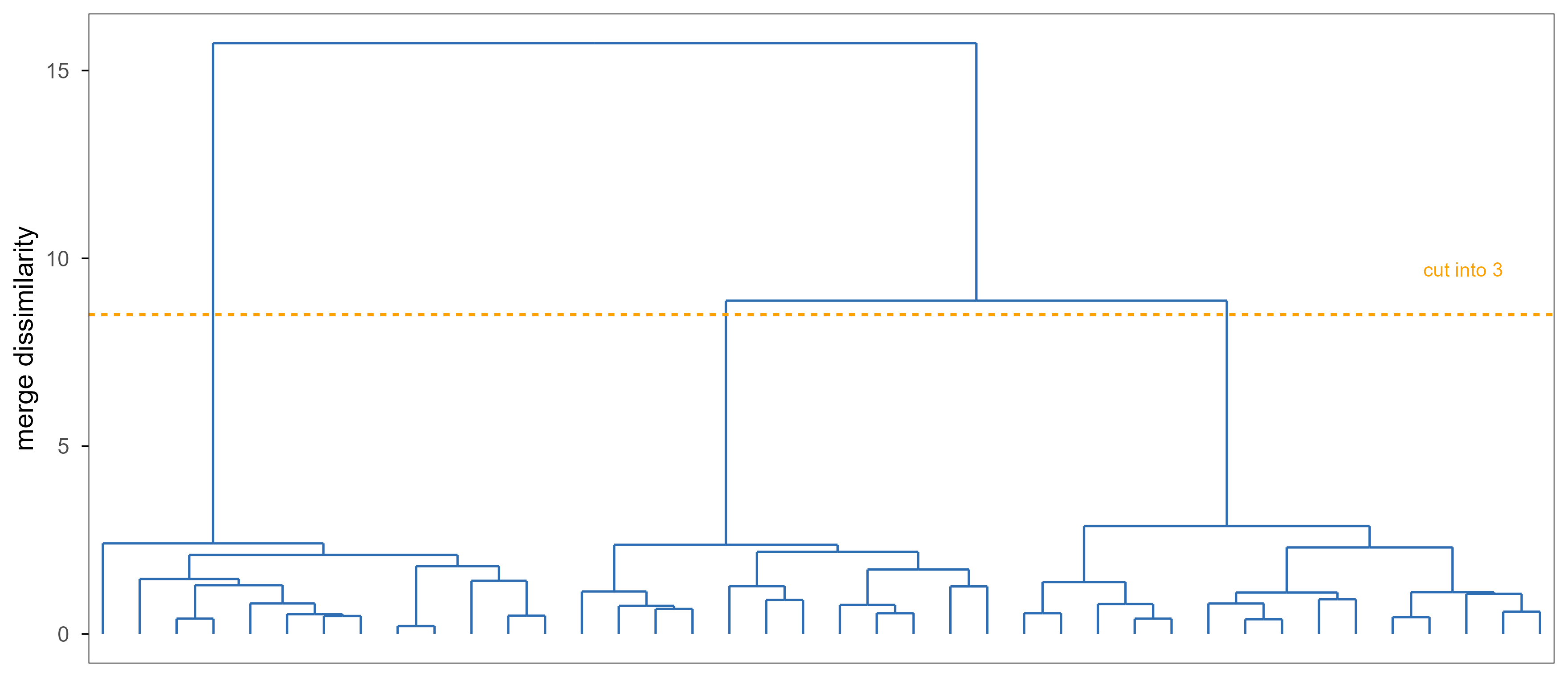
Hierarchical clustering does not decide the number of clusters up front; it builds a tree, merging the closest pair of clusters until one remains. The definition of cluster-to-cluster distance (linkage) changes the tree completely: complete uses the farthest pair, average uses the mean distance, Ward merges where the increase in within-cluster sum of squares is smallest.
Figure 15: 在 40 个样本、5 个变量上的 Ward 层次聚类。纵轴是合并时的不相似度,虚线标出切成 3 簇的位置。树一旦建好,切 2 刀还是 3 刀只是看图决定,不必重新计算——这是它与 K-means 最实用的差别。 | Ward hierarchical clustering on 40 samples and 5 variables. The vertical axis is the dissimilarity at each merge; the dashed line marks the cut that yields three clusters. Once the tree exists, cutting at two or three clusters is a visual decision with no recomputation — the most practical difference from K-means.
The most useful property is that the number of clusters need not be fixed in advance: look at the tree, then decide where to cut. The drawback is that it is also greedy — once two clusters merge they never separate, so an early mistake stays in the tree. Memory is \(O(n^2)\), so tens of thousands of cells are not practical directly.
6.3 高斯混合:把”属于哪一簇”变成概率 / Gaussian mixtures: membership becomes a probability
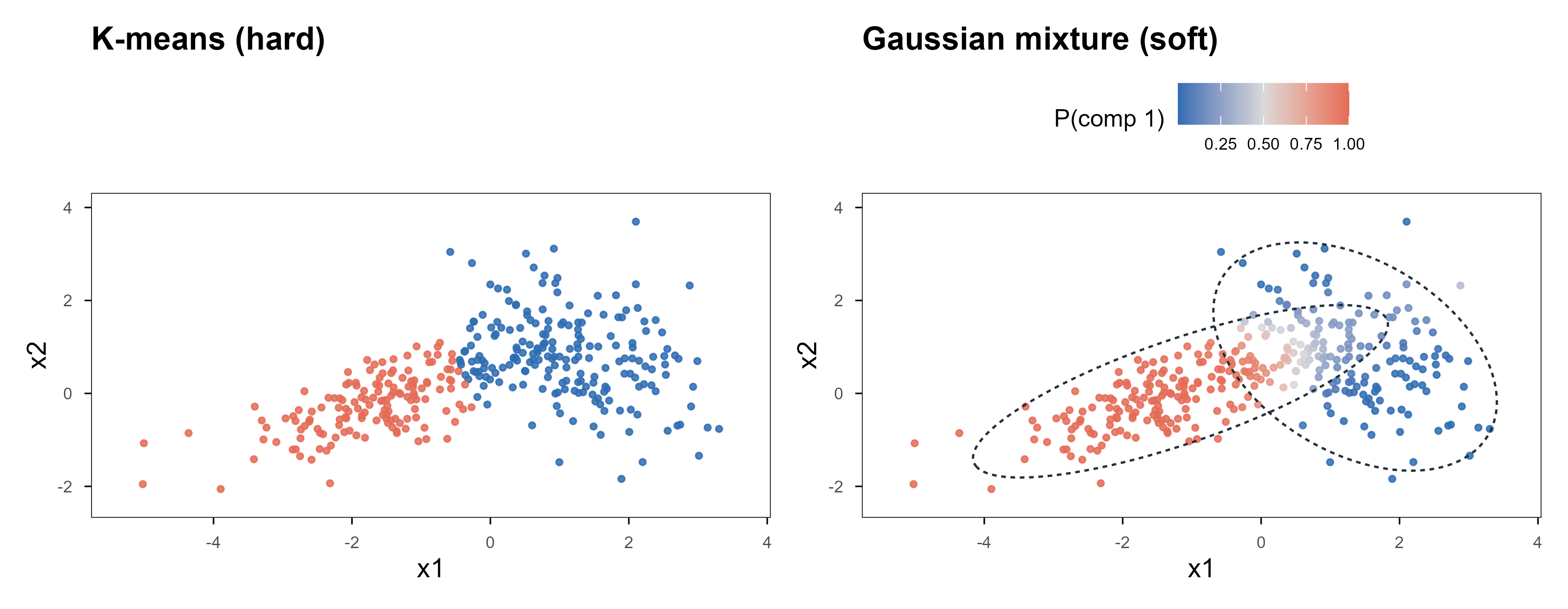
K-means gives each point a hard label. A Gaussian mixture model (GMM) assumes the data come from a mixture of \(K\) Gaussians and outputs a posterior probability:
\(\gamma_{ik}\) is the responsibility of component \(k\) for point \(i\). Parameters are fitted by EM: the E-step computes \(\gamma\), the M-step re-estimates \(\pi,\mu,\Sigma\) with those weights, alternating until the log-likelihood stops rising. Compared with K-means this adds two things: soft assignment and a covariance per component (ellipses, not just circles).
Code
set.seed(20261101)Xg <-rbind( MASS::mvrnorm(200, c(-1.3, 0.0), matrix(c(1.7, 0.75, 0.75, 0.55), 2)), MASS::mvrnorm(150, c( 1.4, 0.9), matrix(c(0.75, -0.4, -0.4, 1.0), 2)))# --- EM for a two-component Gaussian mixture (density written out to avoid a dependency) ---dmv2 <-function(X, mu, S) { Z <-sweep(X, 2, mu) Sinv <-solve(S)exp(-0.5*rowSums((Z %*% Sinv) * Z)) /sqrt((2* pi)^ncol(X) *det(S))}mu <- Xg[sample(nrow(Xg), 2), ]Sig <-list(diag(2), diag(2)); pie <-c(0.5, 0.5)for (it in1:80) { dens <-sapply(1:2, function(k) pie[k] *dmv2(Xg, mu[k, ], Sig[[k]])) gam <- dens /rowSums(dens) Nk <-colSums(gam)for (k in1:2) { mu[k, ] <-colSums(gam[, k] * Xg) / Nk[k] Z <-sweep(Xg, 2, mu[k, ]) Sig[[k]] <-crossprod(sqrt(gam[, k]) * Z) / Nk[k] } pie <- Nk /nrow(Xg)}ell <-function(m, S, lev =0.95) { e <-eigen(S); r <-sqrt(qchisq(lev, df =2)) tt <-seq(0, 2* pi, length.out =240) pts <-t(e$vectors %*% (r *sqrt(e$values) *rbind(cos(tt), sin(tt))))data.frame(x = pts[, 1] + m[1], y = pts[, 2] + m[2])}el <-rbind(cbind(ell(mu[1, ], Sig[[1]]), k ="1"), cbind(ell(mu[2, ], Sig[[2]]), k ="2"))p_gmm <-ggplot() +geom_point(aes(x = Xg[, 1], y = Xg[, 2], colour = gam[, 1]), size =0.9, alpha =0.85) +geom_path(data = el, aes(x, y, group = k), linetype ="22",colour = ml_pal[["ink"]], linewidth =0.45) +scale_colour_gradient2(low = ml_pal[["blue"]], mid ="#D9D9D9", high = ml_pal[["coral"]],midpoint =0.5, name ="P(comp 1)") +coord_cartesian(xlim =range(Xg[, 1]) +c(-0.3, 0.3),ylim =range(Xg[, 2]) +c(-0.3, 0.3)) +labs(x ="x1", y ="x2", title ="Gaussian mixture (soft)") +theme(axis.text =element_text(size =7), legend.key.width =unit(0.5, "cm"),legend.text =element_text(size =7))km <-kmeans(Xg, centers =2, nstart =10)p_km <-ggplot() +geom_point(aes(x = Xg[, 1], y = Xg[, 2], colour =factor(km$cluster)), size =0.9, alpha =0.85) +scale_colour_manual(values =unname(ml_pal[c("blue", "coral")]), guide ="none") +coord_cartesian(xlim =range(Xg[, 1]) +c(-0.3, 0.3),ylim =range(Xg[, 2]) +c(-0.3, 0.3)) +labs(x ="x1", y ="x2", title ="K-means (hard)") +theme(axis.text =element_text(size =7))p_km + p_gmm
Figure 16: 同一批数据,两种模型。左:K-means 只能给出直的分界,两个明显拉长的簇被从中间切开。右:GMM 的软分配,颜色深浅是后验概率,虚线圈是各成分的 95% 椭圆。注意力被放在「哪些点真的模糊」上,而不是被迫押注。 | The same data under two models. Left: K-means can only give a straight cut, slicing two visibly elongated clusters down the middle. Right: GMM’s soft assignment, with colour intensity showing the posterior and dashed rings the 95% ellipses of each component. Attention goes to the points that really are ambiguous instead of being forced into a bet.
The price is many more parameters: each component has \(d(d+1)/2\) covariance entries, which overfits badly in high dimensions, so in practice you regularise (the VEE/VVV model families in mclust exist for exactly this). It also still needs \(K\) from you, though BIC gives a principled way to choose it.
6.4 PCA:找方差最大的方向 / PCA: find the directions of most variance
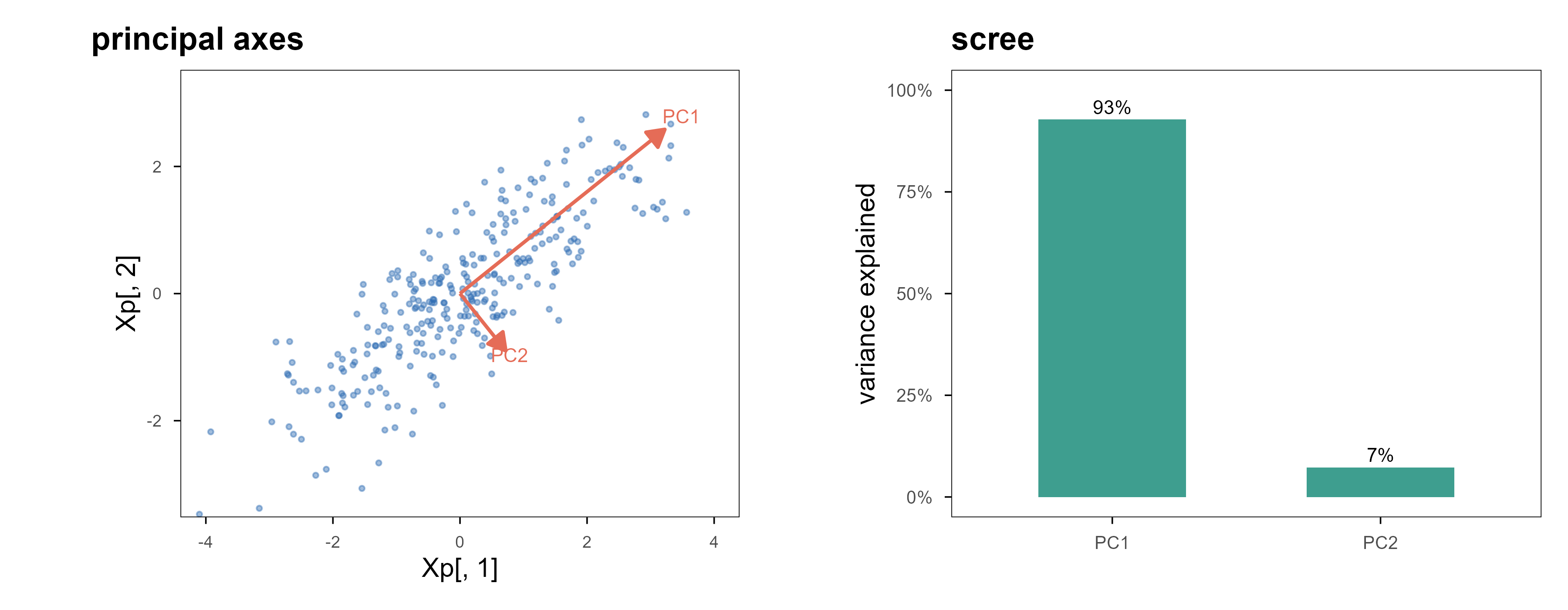
PCA is purely linear: find an orthogonal set of directions such that projections onto them have maximal, decreasing variance. Mathematically it is an eigendecomposition of the covariance matrix.
Figure 17: 左:PCA 的两个主轴,长度正比于该方向的标准差;数据在 PC1 上的投影保留了大部分变化。右:各主成分解释的方差比例,前两个成分合计超过九成,后面的基本是噪声。降维的依据就是这张图,而不是「习惯降到二维」。 | Left: the two principal axes, with lengths proportional to the standard deviation along each; projecting onto PC1 keeps most of the variation. Right: the proportion of variance explained by each component — the first two account for more than ninety percent and the rest is noise. This panel, not habit, is the justification for reducing dimensions.
Two common misuses. First, centring is mandatory, otherwise the first component is dominated by the mean; whether to standardise depends on whether the units are comparable (expression data usually standardised, same-instrument channels possibly not). Second, a component is not a latent variable — it is an orthogonal direction, and calling PC1 “some biological process” needs evidence beyond a large loading.
6.5 t-SNE 与 UMAP:只保证邻域,不保证全局 / t-SNE and UMAP: neighbourhoods, not distances
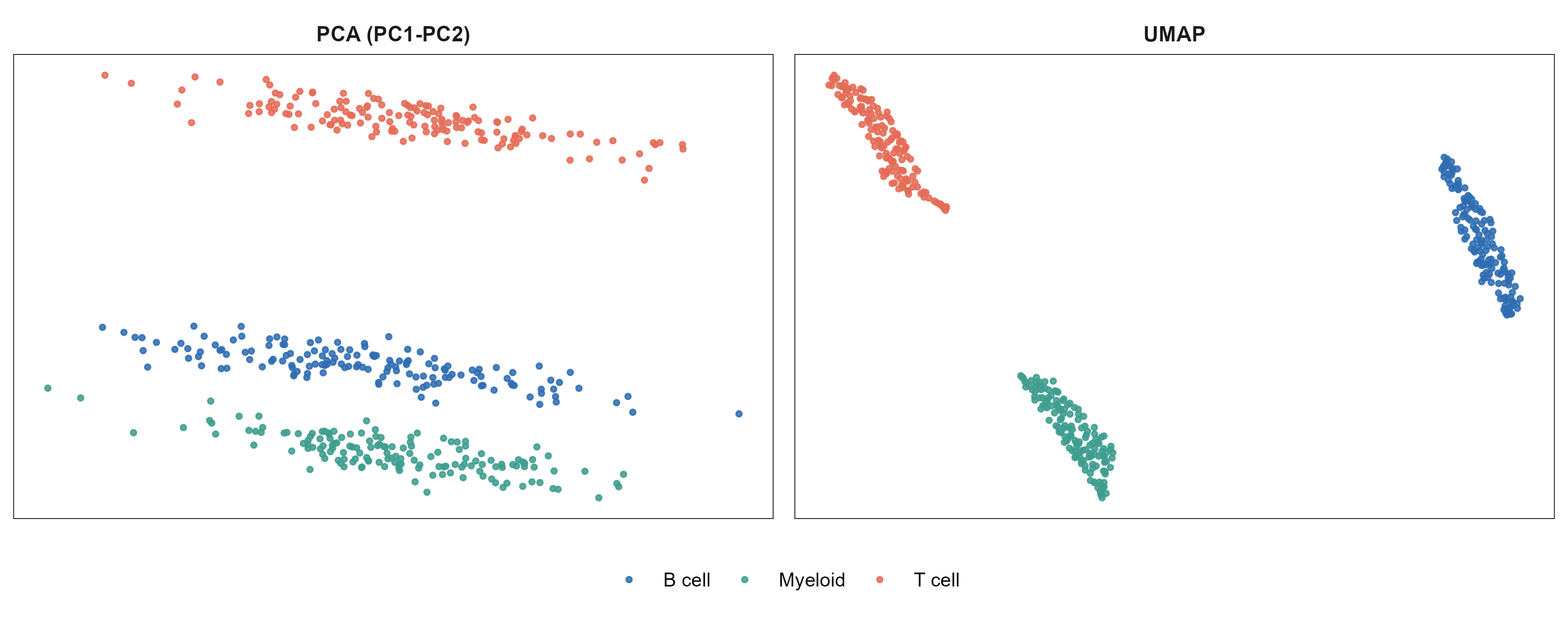
Both are nonlinear embeddings. The goal is not to preserve variance but neighbourhood structure: points that were close stay close in the plane. Each builds a probability distribution over “who is whose neighbour”, then finds a low-dimensional layout whose distribution matches it.
Figure 18: 模拟的 450 个细胞、300 个基因,三类细胞各有 40 个标记基因。左:PCA 前两维,三类已经分开但仍有重叠。右:UMAP,类内更紧凑、类间边界更清晰。两图坐标轴的刻度都没有意义——只能读相对位置。 | 450 simulated cells and 300 genes, with 40 marker genes per cell type. Left: the first two principal components; the three types separate but still overlap. Right: UMAP, tighter within types and cleaner between them. The axis ticks in both panels are meaningless — only relative position can be read.
The most common misreading is treating between-cluster distances as biological distances. UMAP preserves neighbourhoods, so how far apart two clusters sit carries almost no information; change n_neighbors or min_dist and the layout moves while membership barely changes. Use UMAP to ask “are there groups”, then go back to the original space (or PCA) for differential expression and tests. Reading conclusions off UMAP distances is one of the most common errors in the single-cell literature.
Every conclusion in the previous chapters — “this model is better”, “this hyperparameter is optimal” — rests on one thing: the data used for evaluation took no part in fitting. This chapter is about guaranteeing that, and how easily it breaks.
A single hold-out is simplest: split once, fit on one part, evaluate on the other. Its weakness is dependence on that one split, which is noisy when \(n\) is small. \(K\)-fold cross-validation splits the data into \(K\) parts, trains on \(K-1\) and evaluates on the remaining one in turn, then averages — every sample is evaluated exactly once, with much lower variance than a single hold-out.
方案 / Scheme
做法 / How
何时用 / When
留出 / hold-out
一次 70/30 或 80/20 切分
样本多、只想要一个快速估计 / large \(n\), quick estimate
K 折 / k-fold
轮流留出 1 份,\(K=5\) 或 10
默认选择 / the default
分层 K 折 / stratified
每折里类别比例与总体一致
类别不平衡 / imbalanced classes
留一 / leave-one-out
\(K=n\)
极小样本,但方差反而可能更大 / tiny \(n\); variance can be worse
自助法 / bootstrap
有放回抽样,约 63% 的样本被抽中
想估计不确定性 / uncertainty estimates
English
Scheme
How
When
hold-out
one 70/30 or 80/20 split
large \(n\), quick estimate
k-fold
hold out 1 of \(K\) parts, \(K=5\) or 10
the default
stratified
class ratio preserved in each fold
imbalanced classes
leave-one-out
\(K=n\)
tiny \(n\); variance can be worse
bootstrap
sample with replacement, ~63% drawn
uncertainty estimates
7.2 泄漏:最常见、也最不容易察觉的错误 / Leakage: the most common silent error
Writing the loop is easy; keeping each fold self-contained is hard. Any step that touches all the data — standardisation, imputation, dimensionality reduction, feature selection, batch-correction parameters — leaks information from the held-out fold into training and makes the estimate optimistic.
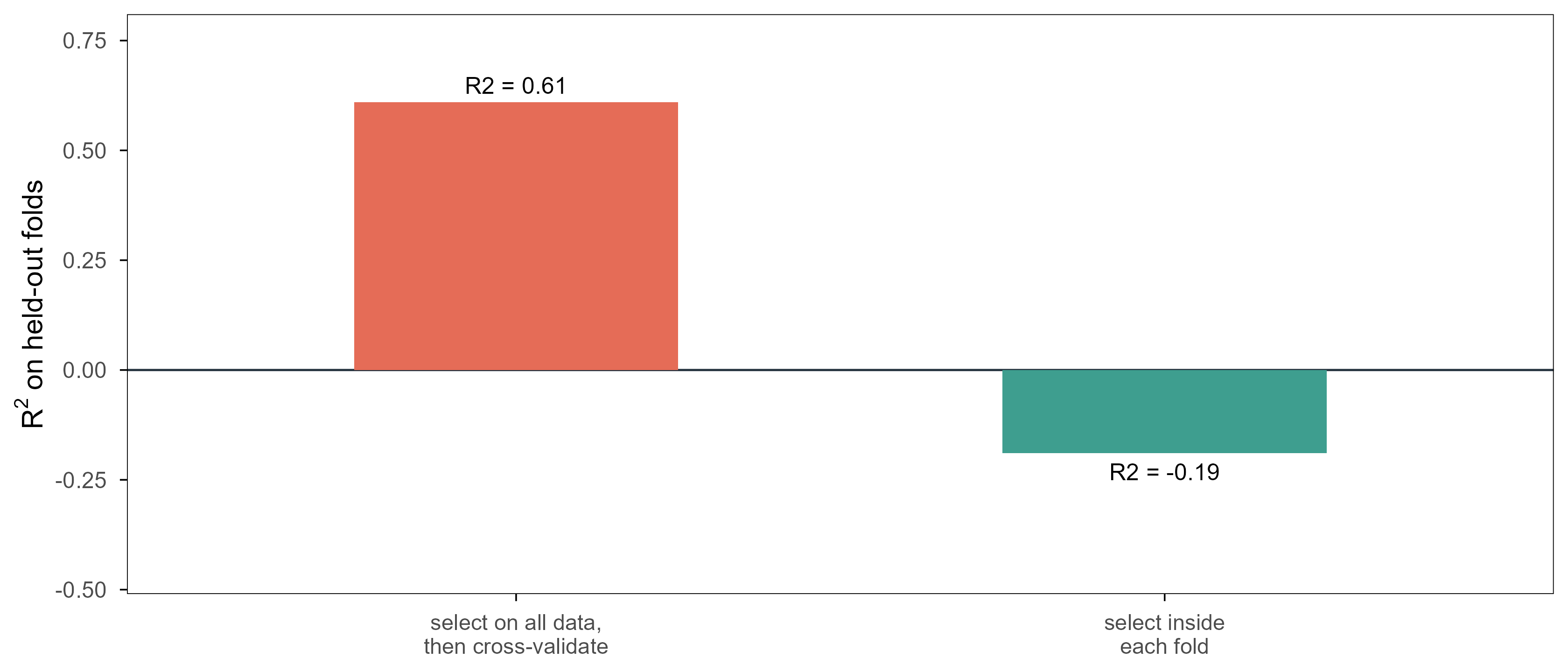
Figure 19: 一次刻意设计的泄漏。60 个样本、5000 个与结局完全无关的随机基因,所以真实的 \(R^2\) 应该是 0。若先在全部数据上挑出与 \(y\) 相关性最强的 20 个基因、再做交叉验证,\(R^2\) 会明显偏高;把挑选放进每一折内部,\(R^2\) 回到 0 附近甚至为负。差别完全来自那一步「提前看了测试集」。 | A deliberately constructed leak. Sixty samples and five thousand random genes with no relation to the outcome, so the true \(R^2\) is 0. Selecting the 20 genes most correlated with \(y\) on all the data and then cross-validating inflates \(R^2\) well above zero; doing the selection inside each fold brings it back to about zero or below. The entire difference comes from one step that 「peeked at the test set」.
The data here are pure noise, so any positive true \(R^2\) is fake. The leaky protocol reports 0.61; the correct one reports -0.19. The negative value is not a bug — it is the correct statement that the model is no better than predicting the mean, and \(R^2\) is allowed to be negative.
Real leaks are subtler: imputing with the whole-cohort mean, running PCA on all samples and keeping ten components, estimating batch effects from everything, doing differential expression before splitting. There is one test: could this step be done independently when a new sample arrives? If yes, it must be redone inside every fold.
7.3 嵌套交叉验证:调参与评估不能共用同一批折 / Nested CV: tuning and evaluation need different folds
如果调参也用交叉验证,再用同一个交叉验证结果报告性能,就犯了和上一节同类的错误:超参数是”看着测试折”选出来的,报告的数字必然偏乐观。正确做法是嵌套:外层 K 折负责评估,每一折内部再做一次内层交叉验证来选超参数。
If tuning also uses cross-validation and you then report that same CV number, you repeat the mistake: the hyperparameter was chosen while looking at the evaluation folds, so the number is optimistic. The fix is nesting: an outer \(K\)-fold loop for evaluation, with an inner cross-validation inside each outer training fold to pick the hyperparameter.
The price is a factor of \(K\) in compute: outer 5 by inner 5 means 25 fits. A common compromise is to use nested CV for one trustworthy performance number, then run ordinary CV on all the data to pick the final hyperparameters.
7.4 三个工作流框架,怎么选 / Three workflow frameworks
caret
tidymodels
mlr3
首次发布 / first release
2007
2018 起逐步成型
2019
设计 / design
一个大 train() 函数
管道与对象组合(recipes + parsnip + workflows)
面向对象的 task / learner / measure
强项 / strength
上手最快,模型最多
流程可读、可版本化,与 tidyverse 一致
批量 benchmark、超参数调优、并行
弱项 / weakness
接口偏老,扩展性一般
概念多,初学门槛高
语法重,小项目显繁琐
适合 / fits
一次性分析、教学
需要长期维护的分析流水线
多数据集、多模型的比较实验
English
caret
tidymodels
mlr3
first release
2007
assembled from 2018
2019
design
one big train()
composable pipes (recipes + parsnip + workflows)
object-oriented task / learner / measure
strength
fastest to start, widest model coverage
readable, versionable pipelines that match the tidyverse
What the three share is that they bind preprocessing, model and resampling into one object, which is exactly the anti-leak mechanism: once preprocessing lives inside the workflow, it is refitted inside every fold automatically. The three snippets in section 1 do the same job and differ only in abstraction. The advice is simple: caret for a one-off analysis, tidymodels for something maintained, mlr3 for benchmarks over dozens of datasets. Do not use all three.
R 版 torch 和 PyTorch 共用同一套 libtorch 后端,所以 API 几乎是镜像的:nn_sequential() 搭网络,loss$backward() 自动求导,optim_adam() 更新参数。下面这段代码是一个真正的训练循环,不是伪代码——它会在本文渲染时实际跑一遍。
R’s torch shares the libtorch backend with PyTorch, so the API mirrors it: nn_sequential() builds the network, loss$backward() differentiates automatically, optim_adam() updates parameters. The code below is a real training loop, not pseudocode — it runs when this page is rendered.
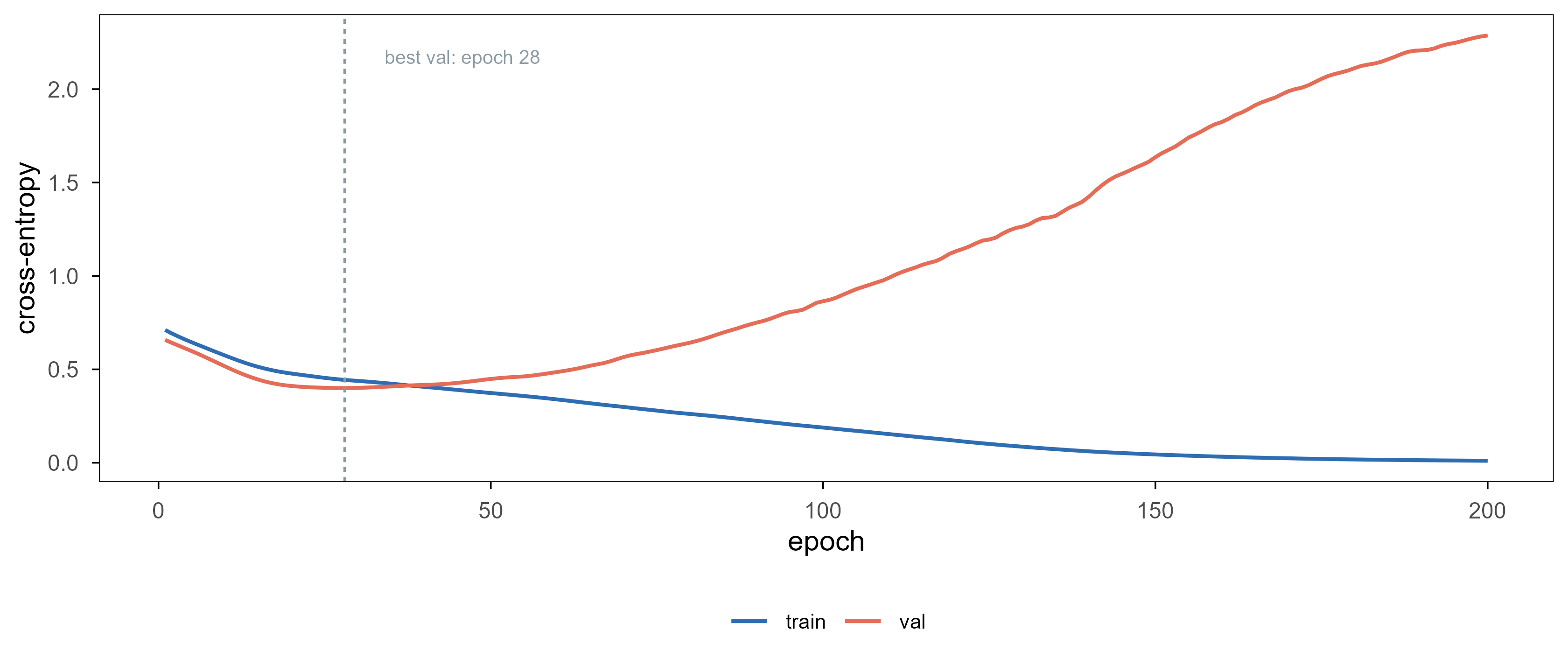
Figure 20: 在 Pima 训练集内部切分出的 140/60 上训练一个 7-16-8-1 的小网络,200 轮,Adam,学习率 0.01。两条曲线都是交叉熵:训练损失单调下降,验证损失在第 28 轮触底后一路回升——这就是过拟合的曲线形状,也是早停的依据。 | A 7-16-8-1 network trained on a 140/60 split inside the Pima training set for 200 epochs with Adam at learning rate 0.01. Both curves are cross-entropy: training loss falls monotonically while validation loss bottoms out at epoch 28 and then climbs — the shape of overfitting, and the justification for early stopping.
这段代码里没有一行是在”实现”反向传播——loss$backward() 一行就完成了。真正的实现藏在 libtorch 里:每个算子都注册了自己的前向计算和反向函数(这正是上一篇讲算子的文章里第 1.4 节的那个要求)。用 R 写深度学习,你写的是计算图,不是梯度公式。
Not one line here “implements” backpropagation — loss$backward() does it. The implementation lives inside libtorch: every operator registers a forward pass and a backward rule (exactly the requirement discussed in section 1.4 of the operators article). Writing deep learning in R means writing computation graphs, not gradient formulae.
8.2 keras3:更高层的封装 / keras3: a higher-level wrapper
keras3 folds the training loop into fit(), which suits quick prototypes; the price is coarser control, and custom losses or complex multi-input models need workarounds.
On tabular data a well-tuned xgboost usually ties or beats a neural network at an order of magnitude less compute — not a prejudice but a repeatedly benchmarked result. Deep learning pulls ahead when several things hold at once: very large samples, high-dimensional raw input (pixels, waveforms, characters, bases), and usable pretraining. Pima has 200 cases and seven variables, satisfying none of them, so the network above is an API demonstration, not a better model.
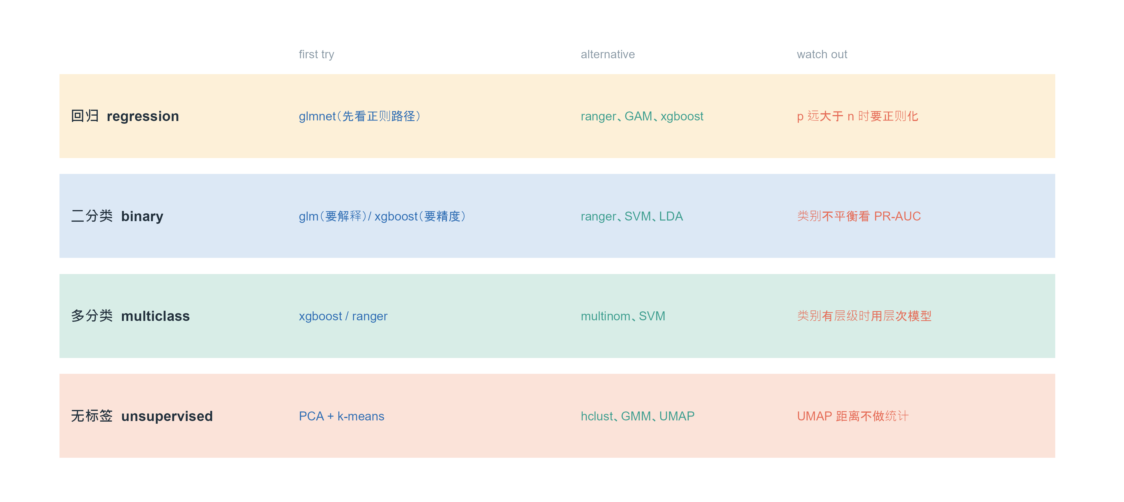
Figure 21: 按任务类型给出的起点建议。左列是问题,中间三列是从「先试什么」到「什么时候不该用」。这不是规则,而是默认起点:任何一行都可能因为样本量、维度或数据结构而被推翻。 | Starting points by task type. The left column is the problem, the next three run from 「try first」 to 「when not to」. These are defaults, not rules: any row can be overturned by sample size, dimensionality or data structure.
选完模型之后,还有八件事决定你的结论可不可信。这份清单可以贴在墙上:
Once the model is chosen, eight things decide whether your conclusion is trustworthy. Pin this list to the wall:
先看数据,再看模型。分布、缺失、异常值、批次;一张 UMAP 或一组箱线图往往比换模型更有用。 Look at the data before the model. Distributions, missingness, outliers, batches; one UMAP or a boxplot often helps more than a new algorithm.
说清楚预测单位是什么。一个样本是一个病人、一个细胞还是一个技术重复?单位错了,交叉验证就错了。 State the unit of prediction. Is a sample a patient, a cell, a technical replicate? Wrong unit, wrong cross-validation.
划分要模拟真实使用。同一病人的多个样本不能分到训练和测试两边;时间序列不能随机打乱。 Split the way the model will be used. Samples from one patient must not straddle train and test; time series must not be shuffled.
预处理必须在折内做。标准化、填补、降维、特征选择,一个都不能提前。 Preprocessing belongs inside the fold. Standardisation, imputation, reduction, selection — none may be done in advance.
报告不确定度。单个 AUC 没有意义,要给置信区间或多个随机种子的分布。 Report uncertainty. A single AUC means little; give a confidence interval or a spread over seeds.
给基线。至少给一个”什么都不做”的基线(预测均值、多数类)和一个简单模型(逻辑回归)。 Always include a baseline: predict the mean or the majority class, plus one simple model.
解释要落在数据上。重要性和 PDP 是描述性的,不是因果的;要说因果得另做设计。 Keep interpretation descriptive. Importance and PDP are not causal; causal claims need a different design.
写下失败的条件。在什么数据上这个方法会失效,比”我们的方法更好”更有信息量。 Write down where it fails. That is more informative than “our method is better”.
参考文献 / References
Hastie, T., Tibshirani, R. & Friedman, J. (2009). The Elements of Statistical Learning (2nd ed.). Springer. https://hastie.su.domains/ElemStatLearn/
James, G., Witten, D., Hastie, T. & Tibshirani, R. (2021). An Introduction to Statistical Learning (2nd ed.). Springer. https://www.statlearning.com
Tibshirani, R. (1996). Regression shrinkage and selection via the lasso. Journal of the Royal Statistical Society B 58, 267–288.
Zou, H. & Hastie, T. (2005). Regularization and variable selection via the elastic net. JRSS B 67, 301–320.
Friedman, J., Hastie, T. & Tibshirani, R. (2010). Regularization paths for generalized linear models via coordinate descent. Journal of Statistical Software 33(1), 1–22.
Breiman, L. (2001). Random forests. Machine Learning 45, 5–32.
Friedman, J. (2001). Greedy function approximation: a gradient boosting machine. Annals of Statistics 29, 1189–1232.
Chen, T. & Guestrin, C. (2016). XGBoost: a scalable tree boosting system. KDD. arXiv:1603.02754
Wright, M. N. & Ziegler, A. (2017). ranger: a fast implementation of random forests for high dimensional data in C++ and R. Journal of Statistical Software 77(1), 1–17.
Cortes, C. & Vapnik, V. (1995). Support-vector networks. Machine Learning 20, 273–297.
Lloyd, S. P. (1982). Least squares quantization in PCM. IEEE Transactions on Information Theory 28, 129–137.
Dempster, A. P., Laird, N. M. & Rubin, D. B. (1977). Maximum likelihood from incomplete data via the EM algorithm. JRSS B 39, 1–38.
van der Maaten, L. & Hinton, G. (2008). Visualizing data using t-SNE. Journal of Machine Learning Research 9, 2579–2605.
McInnes, L., Healy, J. & Melville, J. (2018). UMAP: uniform manifold approximation and projection for dimension reduction. arXiv:1802.03426
Kuhn, M. (2008). Building predictive models in R using the caret package. Journal of Statistical Software 28(5), 1–26.
Kuhn, M. & Wickham, H. (2020). tidymodels: a collection of packages for modeling and machine learning. https://www.tidymodels.org
Lang, M., et al. (2019). mlr3: a modern object-oriented machine learning framework in R. https://mlr-org.com
Paszke, A., et al. (2019). PyTorch: an imperative style, high-performance deep learning library. NeurIPS. arXiv:1912.01703
R Core Team (2025). R: A Language and Environment for Statistical Computing. https://www.R-project.org
Citation note: entries 3–15 and 18 give volume/pages or arXiv identifiers; entries 1, 2, 16, 17 and 19 are books, websites or software home pages — refer to the official pages. Every numeric example in this post is generated by the accompanying code; no third-party data are reused.