Cells in Latent Space: How AI Learns to Represent Biological States

写作说明 / Note

本文由 AI（Trae Agent） 检索、整理并撰写，尚未经过人工逐条校对。所有数字均来自本文自带 R 代码的实际运行结果，代码、模拟数据生成器与结果文件都在文章目录中，可逐条复现。真实数据实验使用 10x Genomics 公开的 PBMC3k 数据集，其细胞类型标签由 marker 打分与 k-means 得到，不是金标准。文中引用均给出 DOI 或官方仓库，但请注意软件版本更新会使具体数值变化。

This article was researched and written by an AI system (Trae Agent) and has not been proofread line by line by a human. Every number below comes from an actual run of the R code shipped with the post (simulator, experiment scripts and result files are all in the post directory). The real-data section uses the public 10x Genomics PBMC3k dataset, where cell-type labels come from marker scoring plus k-means — not from a ground truth. References are given with DOIs or official repositories; exact numbers will drift as software versions change.

生成本文所用的提示词（压缩后） / Prompt used to generate this article (condensed)

写一篇中英逐段对照的长文，主题是「细胞状态的低维表征」。要求：围绕 10 个递进问题（观测维度 vs 内在维度；PCA/UMAP/Diffusion Maps/AE/VAE 各在学什么；距离与方向是否具有生物学意义；跨组学对齐；潜在插值能否模拟分化；什么样的表征支持扰动预测）展开；构造一套 3000 细胞 × 1000 基因、含分支轨迹与批次效应的统一模拟系统，跑 8 组 R 实验（PCA、UMAP 稳定性、流形与轨迹、AE/VAE 训练、潜在插值、非配对 RNA-蛋白对齐、状态依赖扰动、真实数据验证）；至少 12 幅统一风格的图，其中 4 幅可交互；必须展示失败案例与反直觉结果，不得为让某个算法好看而调参；所有数字来自实际运行。

Write a bilingual (paragraph-by-paragraph) long-form article on low-dimensional representations of cell state. Cover ten escalating questions: observed vs intrinsic dimension; what PCA, UMAP, diffusion maps, autoencoders and VAEs each learn; whether distances and directions are biologically meaningful; cross-modality alignment; whether latent interpolation simulates differentiation; what kind of representation supports perturbation prediction. Build one shared simulation (3,000 cells × 1,000 genes, branching trajectory, batch effects) and run eight R experiments, including a real public dataset. Produce at least twelve figures in a consistent style, four of them interactive. Show failures and counter-intuitive results; never tune the simulation so that a preferred method wins; every number must come from a real run.

1. 一个细胞究竟有多少维？ / How Many Dimensions Does a Cell Have?

一个细胞被观测到的样子，是一个长度约两万的向量。单细胞 RNA 测序把每个细胞拆成一列计数：某个基因在某个细胞里被测到 0 次、3 次、或者 1200 次。把这些列堆起来，就得到一个矩阵 \(X \in \mathbb{R}^{N \times G}\)，其中 \(N\) 是细胞数（本文的模拟系统里是 3000），\(G\) 是基因数（1000）。

A cell, as we observe it, is a vector of roughly twenty thousand numbers. Single-cell RNA sequencing turns each cell into a column of counts: a gene is detected zero times, three times, or twelve hundred times. Stacking those columns gives a matrix \(X \in \mathbb{R}^{N \times G}\), with \(N\) cells (3,000 in the simulation below) and \(G\) genes (1,000).

这个矩阵看起来维度极高，但它并不是在 \(G\) 个方向上均匀铺开的。基因受同一套调控程序控制，会一起升高、一起降低；细胞周期让一批基因周期性地起伏；分化让另一批基因单调地打开或关闭。结果是：数据所占据的区域，其有效自由度远小于 \(G\)。

The matrix looks extremely high-dimensional, but it does not fill the gene space evenly. Genes controlled by the same regulatory programme rise and fall together; the cell cycle makes one block oscillate; differentiation switches another block on or off. The consequence is that the region actually occupied by the data has far fewer effective degrees of freedom than \(G\).

这里必须区分三个概念，全文都会反复用到：

Three notions have to be kept apart, and the whole article depends on the distinction:

• 观测维度（observed dimension）：矩阵的列数 \(G\)，也就是我们测了多少个基因。
  The number of columns \(G\): how many genes we measured.
• 内在维度（intrinsic dimension）：数据云局部真正张成的维数 \(d^\*\)，与坐标系无关。
  The local dimension \(d^\*\) of the data cloud itself, independent of coordinates.
• 潜在维度（latent dimension）：我们假设存在、并试图用模型估计的那几个变量 \(z \in \mathbb{R}^{d}\)。
  The few variables \(z \in \mathbb{R}^{d}\) we assume to exist and try to estimate.

三者并不相等。\(d\) 是我们选的（超参数），\(d^\*\) 是数据的性质，\(G\) 是实验的性质。几乎所有关于「降维是否可信」的争论，最后都会落到「你估计的 \(d\) 和真实的 \(d^\*\) 差多少」上。

The three are not equal. \(d\) is a choice (a hyper-parameter), \(d^\*\) is a property of the data, and \(G\) is a property of the experiment. Most arguments about whether a dimensionality reduction is trustworthy eventually reduce to: how far is the estimated \(d\) from the true \(d^\*\)?

1.1 一个可以验证的系统 / A system with a checkable answer

要回答这个问题，我们需要知道 \(d^\*\)。真实数据里没人知道，所以我们从一套生成模型出发：细胞 \(i\) 的状态由三个连续因子决定——分化进程 \(t_i\)、激活程度 \(a_i\)、以及分化方向（分支）\(b_i\)：

To answer that, we need to know \(d^\*\), which nobody knows for real data. So we start from a generative model in which cell \(i\) is controlled by three continuous factors — differentiation time \(t_i\), activation \(a_i\), and lineage choice \(b_i\):

\[ z_i = (t_i,\; a_i,\; s_i), \qquad s_i = w(t_i)\,(2b_i - 1), \qquad w(t) = \frac{1}{1+e^{-(t-0.58)/0.10}} \]

其中 \(s_i\) 是连续的分支坐标。关键在于 \(w(t)\)：它在分化早期接近 0，在 \(t \approx 0.58\) 之后迅速升到 1。这意味着早期细胞的两个分支在表达上完全不可区分，分支不是一开始就被人为分开的标签，而是随着分化逐渐「显形」的方向。

Here \(s_i\) is a continuous branch coordinate. The important part is \(w(t)\): it is near zero early and rises to one after \(t \approx 0.58\). Two early cells on different branches are therefore indistinguishable in expression; the branch is not a label imposed at \(t=0\) but a direction that becomes visible as differentiation proceeds.

表达由负二项分布生成，均值由五个基因模块叠加而成：

Expression is drawn from a negative-binomial distribution whose mean is a sum of five gene modules:

\[ \log \mu_{ig} = \log L_i + \beta_{0g} + f_g(t_i, s_i, a_i, c_i) + \gamma_{g,\, \text{batch}_i}, \qquad X_{ig} \sim \mathrm{NB}(\mu_{ig}, \theta_g) \]

\(f_g\) 包含 140 个随 \(t\) 单调变化的基因、60 个在分化中途短暂脉冲的基因（pulse）、120 个分支特异基因、120 个激活相关基因和 60 个细胞周期基因；\(L_i\) 是测序深度，\(\gamma\) 是批次效应，\(\theta_g\) 控制过离散程度。这个系统里 \(d^\* = 3\)，是已知的。

\(f_g\) contains 140 monotone genes, 60 transiently pulsing genes, 120 branch genes, 120 activation genes and 60 cell-cycle genes; \(L_i\) is sequencing depth, \(\gamma\) is a batch shift and \(\theta_g\) sets overdispersion. In this system \(d^\* = 3\), and we know it.

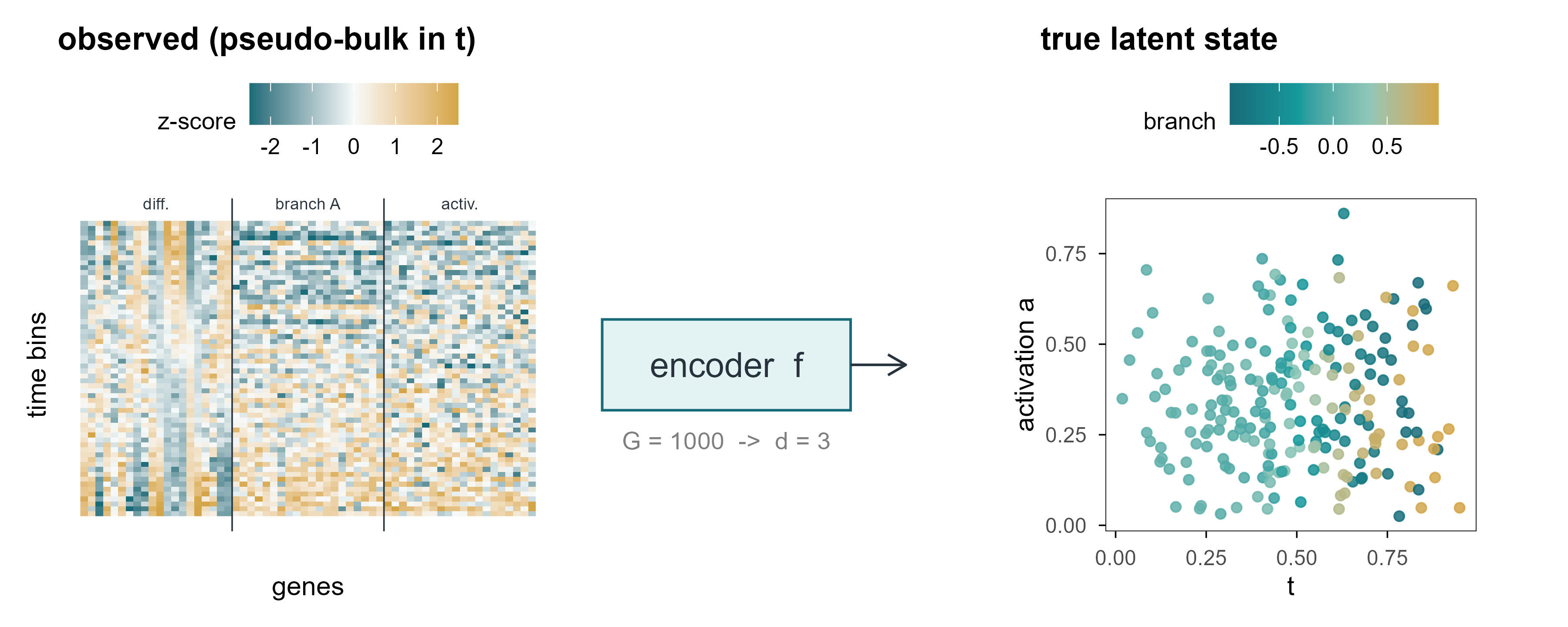
set.seed(1)
sub_genes <- c(sim$modules$mono[1:20], sim$modules$branchA[1:20], sim$modules$activation[1:20])
# pseudo-bulk in 60 bins of differentiation time: averaging reduces counting
# noise so that the underlying modules become visible
Lfull <- as.matrix(logcpm(sim$counts[, sub_genes], lib = Matrix::rowSums(sim$counts)))
o <- order(sim$truth$t)
Lfull <- Lfull[o, ]
grp <- cut(seq_len(nrow(Lfull)), 60, labels = FALSE)
Lbin <- rowsum(Lfull, grp) / as.vector(table(grp))
Lbin <- scale(Lbin)
lt <- tibble(cell = rep(seq_len(60), times = length(sub_genes)),
             gene = rep(seq_along(sub_genes), each = 60),
             value = as.vector(Lbin),
             group = rep(c("differentiation", "branch A", "activation"), each = 20 * 60),
             gene_lab = factor(gene))

p_a <- ggplot(lt, aes(gene, cell, fill = value)) +
  geom_raster() +
  scale_fill_gradient2(low = "#176B78", mid = "#F7FAFA", high = "#D4A547",
                       midpoint = 0, limits = c(-2.5, 2.5), oob = scales::squish,
                       name = "z-score") +
  geom_vline(xintercept = c(20.5, 40.5), colour = cell_pal[["ink"]], linewidth = 0.3) +
  annotate("text", x = c(10.5, 30.5, 50.5), y = 64, label = c("diff.", "branch A", "activ."),
           size = 2.4, colour = cell_pal[["ink"]]) +
  coord_cartesian(ylim = c(0.5, 62)) +
  labs(x = "genes", y = "time bins", title = "observed (pseudo-bulk in t)") +
  theme(axis.text = element_blank(), axis.ticks = element_blank(),
        panel.border = element_blank())

set.seed(1)
sub_cells <- sample(nrow(sim$truth), 220)
z <- sim$truth[sub_cells, ]
p_c <- ggplot(z, aes(Z1, Z2, colour = Z3)) +
  geom_point(size = 1.6, alpha = 0.85) +
  scale_colour_t(name = "branch") +
  labs(x = "t", y = "activation a", title = "true latent state") +
  coord_fixed(ratio = 1)

p_b <- ggplot() +
  annotate("rect", xmin = 0.05, xmax = 0.95, ymin = 0.35, ymax = 0.65,
           fill = "#159A9C", alpha = 0.12, colour = "#176B78") +
  annotate("text", x = 0.5, y = 0.5, label = "encoder  f", size = 5, colour = "#28323C") +
  annotate("segment", x = 0.95, xend = 1.15, y = 0.5, yend = 0.5,
           arrow = arrow(length = unit(3, "mm")), colour = "#28323C") +
  annotate("text", x = 0.5, y = 0.25, label = "G = 1000  ->  d = 3", size = 3.6, colour = "#7F7F7F") +
  coord_cartesian(xlim = c(0, 1.2), ylim = c(0, 1)) +
  theme_void()

(p_a + p_b + p_c) + plot_layout(widths = c(1.1, 0.8, 1.1))

Figure 1: 图 1　从一千维观测到三个隐藏状态。左：3000 个细胞 × 1000 个基因的 log-CPM 子矩阵（仅画 60 个基因）；中：编码器把每个细胞压成 3 维；右：模拟数据真实的潜在空间，颜色为分化进程 \(t\)，形状为分支。 | Figure 1. From a thousand observed dimensions to three hidden states. Left: a log-CPM submatrix of 3,000 cells × 60 of the 1,000 genes. Middle: an encoder maps each cell to three numbers. Right: the simulated ground-truth latent space, coloured by differentiation time \(t\) with branch shown as shape.

1.2 内在维度可以估计，但噪声会骗人 / Intrinsic dimension can be estimated, and noise lies

Levina 与 Bickel 提出的极大似然估计，把每个点周围 \(k\) 个近邻的距离比取倒数：

The Levina–Bickel maximum-likelihood estimator inverts the mean log distance ratio among the \(k\) nearest neighbours of each point:

\[ \hat m_k(x) = \left[\frac{1}{k-1}\sum_{j=1}^{k-1}\log\frac{r_k(x)}{r_j(x)}\right]^{-1} \]

直觉是：在 \(d\) 维空间里，近邻距离随序号大致按 \(r_j \propto j^{1/d}\) 增长，取对数后斜率就是 \(1/d\)。把它用到模拟数据上，结果非常能说明问题。

The intuition: in \(d\) dimensions the neighbour distances grow roughly as \(r_j \propto j^{1/d}\), so the slope on a log scale is \(1/d\). Applying it to the simulation is revealing.

id <- e1$id_est
id$k10 <- round(id$k10, 1); id$k20 <- round(id$k20, 1)
knitr::kable(id, col.names = c("数据 / data", "k = 10", "k = 20"),
             caption = "内在维度的极大似然估计（$k$ 为近邻数）。 | Maximum-likelihood estimate of intrinsic dimension for different neighbour counts.")

Table 1: 内在维度的极大似然估计（\(k\) 为近邻数）。

内在维度的极大似然估计（\(k\) 为近邻数）。 | Maximum-likelihood estimate of intrinsic dimension for different neighbour counts.

数据 / data	k = 10	k = 20
observed, logCPM z-scored	100.0	87.2
observed, depth+batch corrected	113.0	97.5
noiseless expectation (log mu)	3.6	3.6
true factors (t, a, branch)	2.2	2.1

Intrinsic dimension estimates. The generative model has three continuous factors; noise inflates the observed estimate by more than an order of magnitude.

无噪声的期望表达给出 3.6，与设计的 3 个因子相当接近；一旦加上负二项计数噪声，估计值跳到 100 以上。这不是估计器写错了，而是距离集中（distance concentration）：在高维空间里，所有点对的距离趋于相同，近邻距离比 \(r_k/r_j\) 趋于 1，对数趋于 0，倒数就爆掉了。

The noiseless expectation gives 3.6, close to the three designed factors. Add negative-binomial counting noise and the estimate jumps above 100. The estimator is not broken; this is distance concentration: in high dimensions all pairwise distances become similar, the ratios \(r_k/r_j\) approach one, their logs approach zero, and the reciprocal explodes.

这个结果本身就是全文的第一个警告：在单细胞数据上直接估计「有效维度」，得到的是一个由噪声水平决定的数字，而不是生物学的自由度。也正因如此，后面所有方法都必须先做归一化与降噪，再谈维度。

That result is the first warning of the article: estimating “effective dimensionality” directly on single-cell data yields a number set by the noise level, not by biological degrees of freedom. Which is why every method below has to normalise and denoise before any claim about dimension is made.

2. 什么是潜在空间？ / What Is a Latent Space?

假设我们接受「细胞的真实状态由少数变量决定」。那么观测 \(x\) 与状态 \(z\) 的关系可以写成一个两段式映射：先用编码器把观测压到潜在空间，再用解码器把潜在状态还原成观测。

Suppose we accept that the true state of a cell is set by a few variables. The relation between observation \(x\) and state \(z\) is then a two-stage map: an encoder compresses the observation into latent space, and a decoder maps the latent state back to observations.

\[ z = f_\theta(x), \qquad \hat{x} = g_\phi(z) \]

在 PCA 里，\(f_\theta\) 是一个线性投影 \(z = V_d^\top (x - \bar x)\)，\(g_\phi\) 是它的转置 \(V_d z + \bar x\)。在 autoencoder 里，两者都是神经网络。在 VAE 里，\(f_\theta\) 输出的不是一个点，而是一个分布 \(q_\phi(z\mid x)\)。

In PCA, \(f_\theta\) is the linear projection \(z = V_d^\top (x - \bar x)\) and \(g_\phi\) is its transpose. In an autoencoder both are neural networks. In a VAE, \(f_\theta\) outputs not a point but a distribution \(q_\phi(z\mid x)\).

2.1 潜在变量不等于机制 / Latent variables are not mechanisms

这里有一个几乎所有人第一次接触时都会误解的地方。潜在变量是为了让观测的协方差结构变简单而引入的坐标，它不自动对应某个生物学实体。一个潜在维度可能同时混合了细胞周期与测序深度；反过来，一个明确的生物机制（比如某个转录因子）也可能被拆散在两个潜在维度上。

There is a trap almost everyone falls into at first. A latent variable is a coordinate introduced to make the observed covariance structure simpler; it does not automatically correspond to a biological entity. One latent dimension may mix the cell cycle with sequencing depth; conversely, a well-defined mechanism (a transcription factor, say) may be split across two latent dimensions.

区分两种说法很重要：

Two claims must be distinguished:

• 表示性（representational）：存在某个函数 \(f\)，使得 \(z = f(x)\) 能重建 \(x\)，并且在下游任务上有用。这是可检验的。
  There exists a function \(f\) such that \(z=f(x)\) reconstructs \(x\) and is useful downstream. This is testable.
• 因果性（causal）：改变 \(z_j\) 会导致 \(x\) 按某个方向变化，且这种变化在干预下稳定。这需要干预实验，单靠观测数据无法确立。
  Changing \(z_j\) causes \(x\) to move in a specific direction, stably under intervention. This needs perturbation data; observational data alone cannot establish it.

后文第 9、10 章会反复回到这个区分：几乎所有「虚拟细胞」的宣传语，都偷偷把前者当成了后者。

Chapters 9 and 10 return to this distinction repeatedly: most “virtual cell” claims quietly substitute the first for the second.

3. PCA：寻找变化最大的方向 / PCA: Finding the Directions of Maximum Variance

3.1 几何直觉 / Geometric intuition

把细胞画成 \(G\) 维空间里的点。PCA 问的是一个非常朴素的问题：如果只能保留一个方向，哪个方向上的投影能让点散得最开？ 答案是数据协方差矩阵的最大特征向量。第二个方向在与第一个正交的约束下继续最大化剩余方差，依此类推。

Draw each cell as a point in \(G\)-dimensional space. PCA asks a disarmingly simple question: if only one direction can be kept, along which direction is the projection most spread out? The answer is the leading eigenvector of the covariance matrix. The second direction maximises the remaining variance subject to being orthogonal to the first, and so on.

set.seed(7)
n <- 400
rho <- 0.75
Sig <- matrix(c(4, rho * 2 * 0.8, rho * 2 * 0.8, 0.64), 2, 2)
pts <- MASS::mvrnorm(n, c(0, 0), Sig)
ee <- eigen(Sig)
ell <- function(k = 2) {
  th <- seq(0, 2 * pi, length.out = 200)
  cbind(2 * cos(th) * sqrt(ee$values[1]), 2 * sin(th) * sqrt(ee$values[2])) %*%
    t(ee$vectors)
}
el <- as.data.frame(ell())
p_one <- c(2.2, 1.1)
proj <- (p_one %*% ee$vectors[, 1]) %*% t(ee$vectors[, 1])

pA <- ggplot() +
  geom_point(data = as.data.frame(pts), aes(V1, V2), colour = cell_pal[["sky"]],
             alpha = 0.55, size = 1.1) +
  geom_path(data = el, aes(V1, V2), colour = cell_pal[["deep"]], linewidth = 0.6) +
  geom_segment(aes(x = 0, y = 0, xend = ee$vectors[1, 1] * 3.2, yend = ee$vectors[2, 1] * 3.2),
               arrow = arrow(length = unit(2.5, "mm")), colour = cell_pal[["teal"]], linewidth = 0.9) +
  geom_segment(aes(x = 0, y = 0, xend = ee$vectors[1, 2] * 2.4, yend = ee$vectors[2, 2] * 2.4),
               arrow = arrow(length = unit(2.5, "mm")), colour = cell_pal[["gold"]], linewidth = 0.7,
               linetype = "22") +
  geom_point(aes(p_one[1], p_one[2]), colour = cell_pal[["red"]], size = 2.6) +
  geom_segment(aes(x = p_one[1], y = p_one[2], xend = proj[1], yend = proj[2]),
               colour = cell_pal[["red"]], linetype = "dashed", linewidth = 0.4) +
  geom_point(aes(proj[1], proj[2]), colour = cell_pal[["red"]], size = 1.8, shape = 1) +
  labs(x = "gene 1", y = "gene 2", title = "geometry") +
  coord_equal()

scree <- bind_rows(lapply(names(e1$var_explained), function(nm) {
  tibble(pipeline = nm, k = seq_along(e1$var_explained[[nm]]),
         ve = e1$var_explained[[nm]])
}))
pB <- ggplot(scree, aes(k, ve, colour = pipeline)) +
  geom_line(linewidth = 0.6) + geom_point(size = 0.9) +
  scale_y_log10(labels = scales::label_percent(accuracy = 1)) +
  scale_colour_manual(values = unname(cell_pal[c("red", "grey", "sky", "teal", "deep")]), name = NULL) +
  labs(x = "component", y = "variance explained (log scale)",
       title = "variance spectrum")

pc1 <- e1$scores$P0_raw_counts[, 1]
pC <- ggplot(tibble(pc1 = pc1, lib = sim_truth$lib), aes(lib, pc1)) +
  geom_point(size = 0.5, alpha = 0.35, colour = cell_pal[["red"]]) +
  scale_x_log10() +
  labs(x = "library size (log scale)", y = "PC1 of raw counts",
       title = "raw counts: PC1 = depth")

(pA + pB + pC) + plot_layout(widths = c(1, 1, 1))

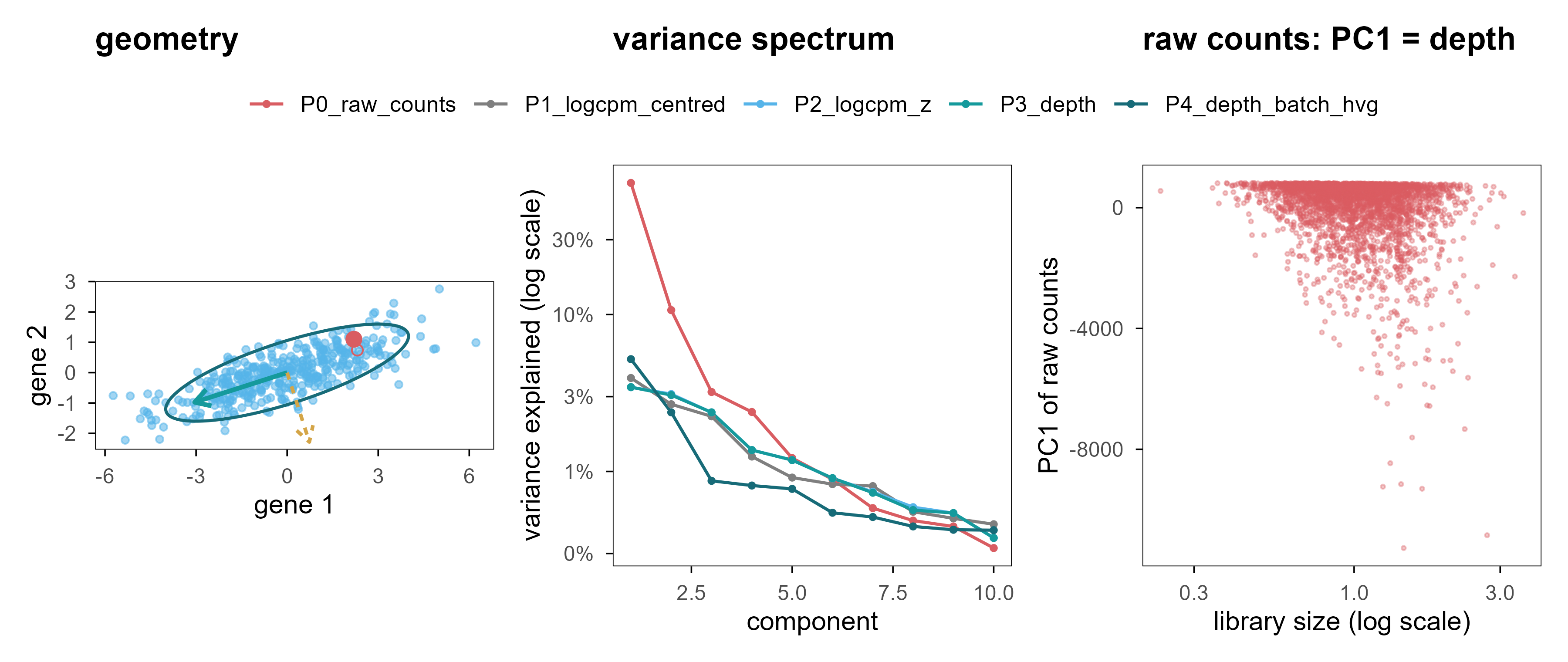
Figure 2: 图 2　PCA 的几何直觉与三个警示。(a) 二维高斯云、协方差椭圆与两条主轴；金色点投影到第一主轴上的位置就是它的 PC1 得分。(b) 五种预处理方案的解释方差谱。(c) 未经文库大小归一化的原始计数：PC1 几乎完全由测序深度决定。 | Figure 2. PCA geometry and three warnings. (a) A bivariate Gaussian cloud with its covariance ellipse and principal axes; the gold point is projected onto PC1. (b) Scree plots for five preprocessing pipelines. (c) Raw counts without library-size normalisation: PC1 is essentially sequencing depth.

PCA geometry (a), the variance spectrum of five pipelines (b), and what happens without normalisation (c).

图 2a 是静态的。下面这张交互图允许你直接改变两个基因的相关性，观察主轴如何旋转、投影点如何移动——这正是 PCA 的全部内容：主轴跟随协方差，而不是跟随任何「意义」。

Figure 2a is static. The interactive version below lets you change the correlation between two genes and watch the principal axes rotate and the projected point move. That is all PCA does: the axes follow the covariance, not any meaning.

rhos <- c(0, 0.7, -0.7)
set.seed(11)
base_pts <- MASS::mvrnorm(300, c(0, 0), diag(2))
pfig <- plot_ly()
vis_list <- list()
for (i in seq_along(rhos)) {
  r <- rhos[i]
  S <- matrix(c(4, r * 1.6, r * 1.6, 0.64), 2, 2)
  ee <- eigen(S)
  P <- base_pts %*% chol(S)
  th <- seq(0, 2*pi, length.out = 120)
  el <- cbind(2*cos(th)*sqrt(ee$values[1]), 2*sin(th)*sqrt(ee$values[2])) %*% t(ee$vectors)
  pfig <- pfig |>
    add_markers(x = P[, 1], y = P[, 2], name = "cells", visible = (i == 1),
                marker = list(size = 3, color = "#56B4E9", opacity = 0.5)) |>
    add_lines(x = el[, 1], y = el[, 2], name = "covariance", visible = (i == 1),
              line = list(color = "#176B78", width = 2), showlegend = FALSE) |>
    add_segments(x = 0, y = 0, xend = ee$vectors[1, 1] * 3.2, yend = ee$vectors[2, 1] * 3.2,
                 name = "PC1", visible = (i == 1),
                 line = list(color = "#159A9C", width = 5), showlegend = FALSE) |>
    add_segments(x = 0, y = 0, xend = ee$vectors[1, 2] * 2.6, yend = ee$vectors[2, 2] * 2.6,
                 name = "PC2", visible = (i == 1),
                 line = list(color = "#D4A547", width = 4), showlegend = FALSE)
  v <- rep(FALSE, 4 * length(rhos)); v[(4 * (i - 1) + 1):(4 * i)] <- TRUE
  vis_list[[i]] <- v
}
pfig <- pfig |> layout(
  title = "gene-gene correlation drives the axes",
  xaxis = list(title = "gene 1", range = c(-8, 8), zeroline = TRUE,
               zerolinecolor = "#cccccc"),
  yaxis = list(title = "gene 2", range = c(-5, 5), zeroline = TRUE,
               zerolinecolor = "#cccccc"),
  paper_bgcolor = "rgba(0,0,0,0)", plot_bgcolor = "rgba(0,0,0,0)",
  updatemenus = list(list(
    type = "buttons", direction = "right", x = 0.5, xanchor = "center", y = 1.15,
    buttons = lapply(seq_along(rhos), function(i) list(
      label = sprintf("rho = %.1f", rhos[i]), method = "update",
      args = list(list(visible = vis_list[[i]]), list(title = sprintf("gene-gene correlation = %.1f", rhos[i])))))
  ))
)
pfig

Figure 3: 图 2b（交互）　点击按钮切换基因间相关性，观察协方差椭圆与主轴的旋转。 | Figure 2b (interactive). Switch the gene-gene correlation and watch the covariance ellipse and principal axes rotate.

3.2 从 SVD 推导 / Derivation via the SVD

把去中心化的矩阵记作 \(X_c \in \mathbb{R}^{N\times G}\)。它的奇异值分解是

Write the column-centred matrix as \(X_c \in \mathbb{R}^{N\times G}\). Its singular value decomposition is

\[ X_c = U \Sigma V^\top, \qquad U^\top U = I_N,\; V^\top V = I_G,\; \Sigma = \mathrm{diag}(\sigma_1 \ge \sigma_2 \ge \dots) \]

由于 \(X_c^\top X_c = V \Sigma^2 V^\top\)，\(V\) 的列就是协方差矩阵的特征向量，\(\sigma_k^2 / (N-1)\) 就是第 \(k\) 个主成分的方差。于是主成分得分与投影都是同一个东西：

Because \(X_c^\top X_c = V\Sigma^2V^\top\), the columns of \(V\) are eigenvectors of the covariance matrix and \(\sigma_k^2/(N-1)\) is the variance of component \(k\). Scores and projection are then the same operation:

\[ Z_d = X_c V_d, \qquad \hat X_c = Z_d V_d^\top \]

这解释了为什么 PCA 的「编码器」是一个线性映射，也解释了它的根本局限：它只能沿直线方向压缩。如果数据躺在一个弯曲的流形上，任何一条直线方向都只能捕获这个流形的一小段。

This explains both why the PCA “encoder” is a linear map and its fundamental limitation: it can only compress along straight directions. If the data lie on a curved manifold, any straight direction captures only a small piece of it.

3.3 实验 1：方差解释率不等于状态恢复 / Experiment 1: variance explained is not state recovery

我们在同一个模拟系统上比较五种预处理方案，指标统一定义为：ve3 是前三个主成分的解释方差；rec_err3 是留出细胞上用 3 个主成分重建的相对误差；r_t、r_a、r_branch 是前五个主成分与真实因子 \(t, a, s\) 的最大绝对 Spearman 相关；knn 是主成分空间与真实潜在空间中 10 近邻的重合率。

We compare five preprocessing pipelines on the same simulation. ve3 is the variance explained by three components; rec_err3 is the relative reconstruction error on held-out cells; r_t, r_a, r_branch are the largest absolute Spearman correlations between the first five components and the true factors \(t, a, s\); knn is the overlap of 10-nearest-neighbour sets between the component space and the true latent space.

m <- e1$metrics
tab <- data.frame(
  `方案 / pipeline` = m$pipeline,
  `ve3` = sprintf("%.3f", m$ve3),
  `rec_err3` = sprintf("%.3f", m$rec_err3),
  `r_t` = sprintf("%.2f", m$r_t),
  `r_a` = sprintf("%.2f", m$r_a),
  `r_branch` = sprintf("%.2f", m$r_branch),
  `kNN` = sprintf("%.2f", m$knn),
  check.names = FALSE
)
knitr::kable(tab, caption = "五种预处理方案的 PCA 指标。 | PCA metrics for five preprocessing pipelines.")

Table 2: 五种预处理方案的 PCA 指标。 | PCA metrics for five preprocessing pipelines.

方案 / pipeline	ve3	rec_err3	r_t	r_a	r_branch	kNN
P0_raw_counts	0.829	0.438	0.70	0.04	0.41	0.10
P1_logcpm_centred	0.089	0.956	0.92	0.92	0.98	0.12
P2_logcpm_z	0.089	0.957	0.91	0.93	0.98	0.12
P3_depth	0.089	0.957	0.92	0.92	0.98	0.12
P4_depth_batch_hvg	0.084	0.958	0.93	0.84	0.97	0.14

最刺眼的一行是第一行。不作文库大小归一化时，三个主成分解释了 82.9% 的方差，重建误差只有 0.44，但它对 \(t\) 的恢复只有 0.70，对激活状态几乎为零。 原因很直白：原始计数的总方差中，绝大部分是「测序深度 × 基因长度」这类技术因素，PCA 忠实地找到了方差最大的方向——只是那个方向不是生物学。

The first row is the uncomfortable one. Without library-size normalisation, three components explain 82.9% of the variance with a reconstruction error of only 0.44, yet recovery of \(t\) is 0.70 and recovery of activation is essentially zero. The reason is simple: in raw counts, most of the total variance is technical — depth times gene length — and PCA faithfully finds the direction of maximum variance. That direction is just not biology.

这正是本文想反复强调的第一个教训：“解释了多少方差” 是相对于总方差而言的，而总方差里可以几乎不含生物学信号。

This is the first lesson the article keeps returning to: “variance explained” is relative to the total variance, and the total variance may contain almost no biological signal.

归一化之后，前三个主成分分别对应分支、分化进程与激活状态。值得注意的是，它们的顺序与「生物学重要性」无关：分支基因的效应在 \(t\) 较大时被 \(w(t)\) 放大，方差反而最大。同样重要的是它们的量级：三个成分加起来只有 8.9% 的方差，剩下 90% 以上是计数噪声。

After normalisation, the first three components line up with branch, differentiation time and activation. Two things are worth noting. First, their order has nothing to do with biological importance: the branch effect is amplified by \(w(t)\) at late times, so it carries the most variance. Second, their magnitude: together the three components explain only 8.9% of the variance; the remaining 90-odd percent is counting noise.

3.4 一个可监督的上限 / A supervised ceiling

如果所有非监督方法都只拿到 knn ≈ 0.12–0.15，这是方法的问题还是数据的问题？我们用「作弊」的方式给出一个上限：把 \((t, a, s)\) 直接对表达矩阵做线性回归，用拟合值作为嵌入。

If every unsupervised method reaches only knn ≈ 0.12-0.15, is that the method’s fault or the data’s? We cheat to get a ceiling: regress \((t, a, s)\) linearly on the expression matrix and use the fitted values as an embedding.

orc <- e1$oracle
data.frame(
  `指标 / metric` = c("R² (t)", "kNN 重合率 / preservation", "距离相关 / distance correlation"),
  `监督上限 / supervised ceiling` = c(sprintf("%.2f", orc["r2_t"]), sprintf("%.2f", orc["knn"]),
                                      sprintf("%.2f", orc["dist_cor"]))
) |> knitr::kable(caption = "监督学习的近邻保持上限。 | Neighbourhood-preservation ceiling with supervision.")

Table 3: 监督学习的近邻保持上限。 | Neighbourhood-preservation ceiling with supervision.

指标…metric	监督上限…supervised.ceiling
R² (t)	0.97
kNN 重合率 / preservation	0.27
距离相关 / distance correlation	0.88

即使允许模型直接看到答案，10 近邻重合率也只有 0.27。这说明 0.12–0.15 与这个上限的差距，主要来自测量噪声，而不是降维算法的无能。这句话有两个方向的含义：一方面，我们不该用 0.13 与 0.15 之间的差异来宣称某个方法更好；另一方面，任何声称能在单细胞数据上「完美恢复细胞状态」的方法，都值得怀疑。

Even with the answer in hand, 10-nearest-neighbour overlap reaches only 0.27. So the gap between 0.12-0.15 and this ceiling is mostly measurement noise, not algorithmic weakness. That cuts both ways: we should not claim one method beats another on a 0.13-versus-0.15 difference, and we should be suspicious of any claim that a method “perfectly recovers cell state” from single-cell data.

3.5 敏感性分析：批次效应何时接管 / When does a batch effect take over?

主模拟里的批次效应是刻意温和的。把同样的生成器重跑一次，把批次偏移放大三倍，情况立刻改变：

The batch effect in the main simulation is deliberately mild. Re-running the same generator with a three-fold stronger batch shift changes the picture immediately:

knitr::kable(transform(e1$sens_batch,
  batch_r2_pc15 = sprintf("%.2f", batch_r2_pc15),
  r_t = sprintf("%.2f", r_t), ve1 = sprintf("%.3f", ve1)),
  col.names = c("阶段 / stage", "批次 R²（PC1–5）", "r_t", "PC1 方差"),
  caption = "强批次效应下的主成分。 | Leading components under a strong batch effect.")

Table 4: 强批次效应下的主成分。 | Leading components under a strong batch effect.

阶段 / stage	批次 R²（PC1–5）	r_t	PC1 方差
batch effect present	0.98	0.92	0.144
batch centred	0.00	0.74	0.036

批次效应出现时，PC1 上有 98% 的方差可以由批次解释，PC1 的方差占比从 3.0% 左右跳到 14.4%。更微妙的是第二行：简单地对每个批次做中心化，批次 R² 归零，但 \(t\) 的恢复从 0.92 掉到 0.74。批次校正不是免费的——当批次与状态部分混杂时，减掉批次均值也减掉了一部分真实信号。

With the batch effect present, 98% of PC1’s variance is explained by batch, and PC1’s share jumps from about 3.0% to 14.4%. The subtler point is the second row: simple per-batch centring drives the batch R² to zero, but recovery of \(t\) falls from 0.92 to 0.74. Batch correction is not free — when batch is partly confounded with state, subtracting batch means also subtracts real signal.

4. UMAP：高维世界的局部地图 / UMAP: A Local Map of a High-Dimensional World

UMAP 与前文所有方法的不同之处在于，它不试图保留全局距离。它先在高维空间里为每个细胞构造一个模糊的局部邻域图，再在低维空间中寻找一个尽量保持这张图的布局。也就是说，它优化的对象是「邻居关系」，不是「距离」。

What sets UMAP apart is that it does not try to preserve global distances. It first builds a fuzzy local neighbour graph in the high-dimensional space, then searches for a low-dimensional layout that best preserves that graph. Its objective is about neighbourhood relations, not distances.

4.1 算法在优化什么 / What the algorithm optimises

高维侧，对每个点 \(i\)，用指数核定义条件概率并做对称化：

On the high-dimensional side, for each point \(i\) an exponential kernel defines a conditional probability, which is then symmetrised:

\[ p_{j\mid i} = \exp\!\left(-\frac{d(x_i,x_j)-\rho_i}{\sigma_i}\right), \qquad p_{ij} = \frac{p_{j\mid i}+p_{i\mid j}}{2N} \]

其中 \(\rho_i\) 是到最近邻的距离（保证局部连通），\(\sigma_i\) 由「有效近邻数」\(k\) 反解。低维侧用一条重尾曲线 \(q_{ij} = (1 + a\lVert y_i - y_j\rVert^{2b})^{-1}\)，损失是两者的交叉熵：

Here \(\rho_i\) is the distance to the nearest neighbour (which guarantees local connectivity) and \(\sigma_i\) is solved so that the effective neighbour count equals \(k\). On the low-dimensional side a heavy-tailed curve \(q_{ij} = (1 + a\lVert y_i-y_j\rVert^{2b})^{-1}\) is used, and the loss is their cross-entropy:

\[ \mathcal{L} = \sum_{i\neq j} \left[ p_{ij}\log\frac{p_{ij}}{q_{ij}} + (1-p_{ij})\log\frac{1-p_{ij}}{1-q_{ij}}\right] \]

第一项拉近高维邻居，第二项把非邻居推开。\(b\) 控制重尾程度，也就控制了「簇与簇之间能挤多近」——这正是 min_dist 在调节的东西。

The first term attracts high-dimensional neighbours, the second repels non-neighbours. The exponent \(b\) controls how heavy the tail is, hence how tightly clusters may pack — that is what min_dist tunes.

4.2 九个不同的世界 / Nine different worlds

grid_df <- bind_rows(lapply(names(e2$embeddings), function(k) {
  if (k == "genes_direct") return(NULL)
  tibble(key = k, U1 = e2$embeddings[[k]][, 1], U2 = e2$embeddings[[k]][, 2],
         t = e2$truth$t)
}))
lab <- e2$metrics |> filter(key != "genes_direct") |>
  arrange(n_neighbors, min_dist) |>
  mutate(label = sprintf("k=%d, min_dist=%.2f\nkNN %.2f | rho(t) %.2f",
                         n_neighbors, min_dist, knn, r_t),
         label = factor(label, levels = label))
grid_df <- left_join(grid_df, lab[, c("key", "label")], by = "key")

ggplot(grid_df, aes(U1, U2, colour = t)) +
  geom_point(size = 0.25, alpha = 0.8) +
  scale_colour_t(name = "t") +
  facet_wrap(~ label, nrow = 3, scales = "free") +
  labs(x = NULL, y = NULL)

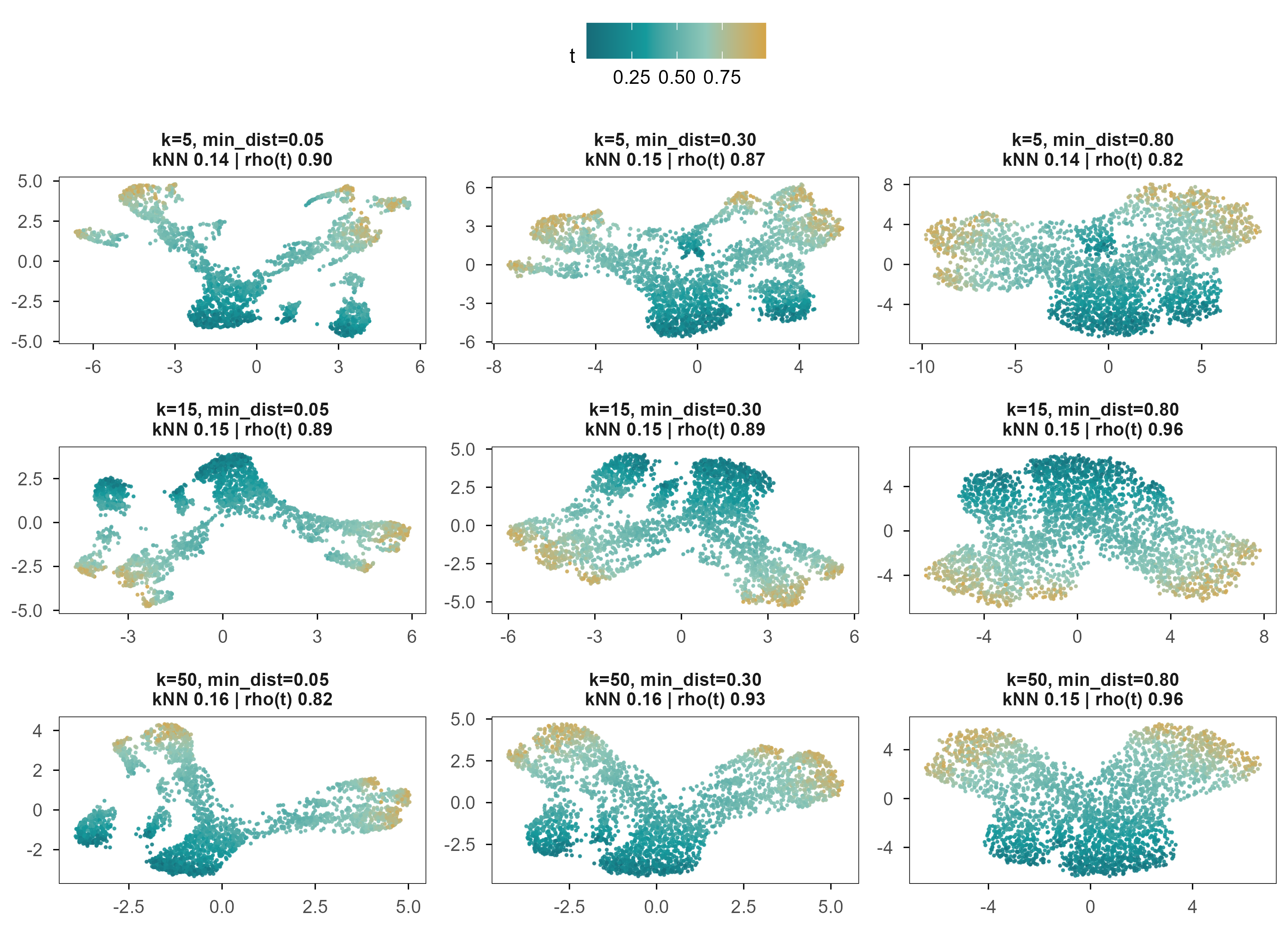
Figure 4: 图 3　同一批细胞、同一份预处理、九组 UMAP 参数。颜色为真实分化进程 \(t\)，面板标题给出该参数下的 10 近邻保持率与 \(t\) 的 Spearman 相关。 | Figure 3. The same cells, the same preprocessing, nine UMAP settings. Colour is the true differentiation time \(t\); panel titles give 10-nearest-neighbour preservation and the Spearman correlation with \(t\).

九个面板看起来都很「好」：连续的色带、清晰的分叉。但它们的邻居保持率几乎一样（0.13–0.16），与 \(t\) 的相关性则从 0.82 波动到 0.96。也就是说，参数选择主要改变的是「看起来像什么」，而不是「保留了多少信息」。

All nine panels look “good”: a continuous colour gradient, a clear bifurcation. Yet their neighbourhood preservation is nearly identical (0.13-0.16), while the correlation with \(t\) ranges from 0.82 to 0.96. In other words, the parameters mainly change what it looks like, not how much information it keeps.

4.3 稳定性：随机种子与重采样 / Stability: seeds and subsampling

stab <- e2$stability
data.frame(
  `扰动 / perturbation` = c("随机种子 1 vs 2", "随机种子 1 vs 3", "随机种子 2 vs 3",
                            "80% 重采样", "直接输入基因 vs 先做 50 个 PC"),
  `Procrustes 相似度 / similarity` = sprintf("%.3f", c(stab$seed_sim, stab$subsample_sim, stab$raw_vs_pc))
) |> knitr::kable(caption = "UMAP 布局在不同扰动下的稳定性（1 = 完全一致）。 | Stability of the UMAP layout under perturbation (1 = identical).")

Table 5: UMAP 布局在不同扰动下的稳定性（1 = 完全一致）。 | Stability of the UMAP layout under perturbation (1 = identical).

扰动…perturbation	Procrustes.相似度…similarity
随机种子 1 vs 2	0.970
随机种子 1 vs 3	0.985
随机种子 2 vs 3	0.954
80% 重采样	0.775
直接输入基因 vs 先做 50 个 PC	0.921

同一个数据、同一个参数、只换随机种子，布局的 Procrustes 相似度是 0.954–0.985；去掉 20% 的细胞，相似度降到 0.775。这比很多人预期的要稳定，但稳定不等于正确：一个稳定地扭曲了距离的映射，依然会稳定地误导你。

Same data, same parameters, different random seed: Procrustes similarity of the layouts is 0.954-0.985. Drop 20% of the cells and it falls to 0.775. That is more stable than many people expect, but stability is not correctness: a map that consistently distorts distances will consistently mislead you.

4.4 距离与簇间距的失真 / Distortion of distance and separation

在模拟数据里，真实的分支轮廓系数是 0.66。UMAP 在九组参数下的轮廓系数是 0.76–0.87，全部高于真值，最高的一组把分支之间的分离度放大了约 1.3 倍。这解释了为什么 UMAP 图上「簇分得很开」：那是优化目标的结果，不是生物学。

In the simulation, the true silhouette of the branch labels is 0.66. Across the nine settings UMAP gives 0.76-0.87, all above the truth, with the most extreme setting inflating branch separation by roughly 1.3-fold. This is why clusters look so far apart in a UMAP plot: it is a consequence of the objective, not of the biology.

因此本文的立场很明确：UMAP 是探索性可视化工具，不是细胞状态的生成模型，也不应被用来比较簇间距离。 下一章我们会看到，若要在意「沿流形的距离」，应该显式地建模流形本身。

Hence the position of this article: UMAP is an exploratory visualisation tool, not a generative model of cell state, and it should not be used to compare distances between clusters. The next chapter shows that if you care about distances along the manifold, you should model the manifold explicitly.

5. 细胞状态真的位于流形上吗？ / Do Cellular States Lie on a Manifold?

「流形假设」是几乎所有单细胞降维方法隐含的前提：高维观测并不是在一个 \(G\) 维盒子里均匀分布，而是集中在一个低维的、可能弯曲的曲面上。分化轨迹是最直观的例子——细胞沿着一条连续的路径从干细胞走向终末状态，路径本身在表达空间中弯弯曲曲。

The manifold hypothesis is the implicit premise of almost every single-cell dimensionality-reduction method: high-dimensional observations are not spread through a \(G\)-dimensional box but concentrate on a low-dimensional, possibly curved surface. A differentiation trajectory is the clearest example — cells move along a continuous path from progenitors to terminal states, and the path itself is curved in expression space.

5.1 卷曲的空间 / A rolled-up space

Swiss roll 是检验这类方法的经典例子：一个二维平面被卷成三维螺旋。数据的内在维度是 2，但任何线性投影都会把不同层叠在一起。

The Swiss roll is the classical test: a two-dimensional sheet rolled into a three-dimensional spiral. The intrinsic dimension is 2, but any linear projection superimposes different layers.

sw <- e3$swiss
plot_ly(x = sw$data[, 1], y = sw$data[, 2], z = sw$data[, 3],
        color = sw$truth$curve, colors = grad_teal_gold,
        type = "scatter3d", mode = "markers",
        marker = list(size = 1.6, opacity = 0.85)) |>
  layout(scene = list(xaxis = list(title = ""), yaxis = list(title = ""),
                      zaxis = list(title = ""), aspectmode = "cube"),
         paper_bgcolor = "rgba(0,0,0,0)")

Figure 5: 图 4a（交互）　Swiss roll：拖动旋转，可见相邻层在三维中靠得很近、在参数空间中却相距很远。颜色为真实曲线位置。 | Figure 4a (interactive). The Swiss roll: drag to rotate. Adjacent layers are close in 3-D but far apart along the underlying parameter. Colour is the true position along the curve.

sw_long <- bind_rows(
  tibble(method = "PCA", D1 = sw$pca[, 1], D2 = sw$pca[, 2], curve = sw$truth$curve),
  tibble(method = "UMAP", D1 = sw$umap[, 1], D2 = sw$umap[, 2], curve = sw$truth$curve),
  tibble(method = "Diffusion map", D1 = sw$dm[, 1], D2 = sw$dm[, 2], curve = sw$truth$curve)
)
lab <- sw$metrics |> mutate(label = sprintf("%s\ngoos = %.2f", method, geo_cor))
sw_long <- left_join(sw_long, lab[, c("method", "label")], by = "method")
ggplot(sw_long, aes(D1, D2, colour = curve)) +
  geom_point(size = 0.45, alpha = 0.85) +
  scale_colour_t(name = "curve") +
  facet_wrap(~ label, scales = "free", nrow = 1) +
  labs(x = NULL, y = NULL)

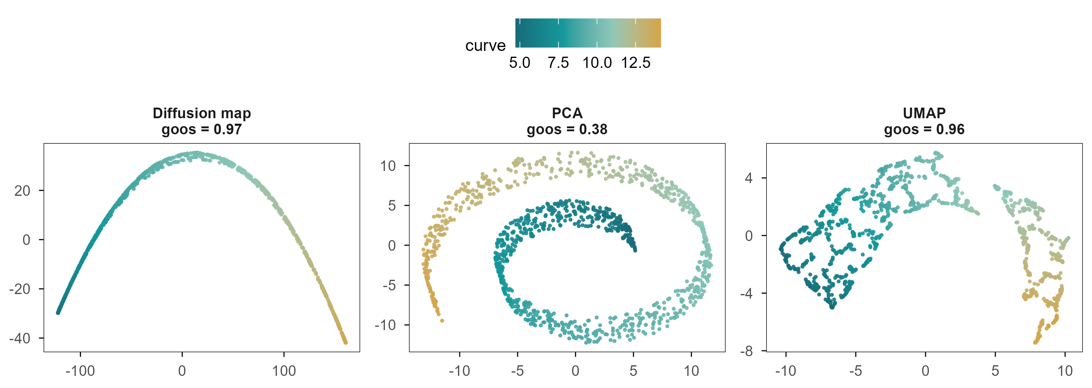
Figure 6: 图 4b　同一个 Swiss roll 的三种二维展开。颜色为真实曲线位置；标题给出二维距离与图测地距离的 Spearman 相关。 | Figure 4b. Three two-dimensional unfoldings of the same Swiss roll. Colour is the true position along the curve; titles give the Spearman correlation between 2-D distance and graph-geodesic distance.

三者的差别不是「好看程度」，而是是否保持了沿流形的距离。Swiss roll 上两点的真实距离是沿曲面的弧长；在二维嵌入里，我们只能用欧氏距离去近似它。用图上最短路作为测地距离的代理，三种方法与它的 Spearman 相关分别是 PCA 0.38、UMAP 0.96、Diffusion Map 0.97。

The difference between the three is not cosmetic; it is whether distances along the manifold are preserved. The true distance between two points on a Swiss roll is arc length along the sheet, which a 2-D embedding can only approximate with Euclidean distance. Using shortest paths on a k-nearest-neighbour graph as a proxy for geodesic distance, the Spearman correlations are 0.38 for PCA, 0.96 for UMAP and 0.97 for diffusion maps.

5.2 Diffusion map：把「随机游走」变成坐标 / Turning a random walk into coordinates

Diffusion map 的思路与前两者都不同。它在数据上定义一个马尔可夫链：从细胞 \(i\) 出发，以与相似度成正比的概率跳到邻居 \(j\)。然后用这个随机游走的多尺度结构作为坐标。

Diffusion maps take a different route. They define a Markov chain on the data: starting from cell \(i\), jump to neighbour \(j\) with probability proportional to their similarity. The multiscale structure of that random walk then becomes the coordinate system.

具体地，用自适应高斯核构造相似度矩阵，再做 \(\alpha = 1\) 的归一化：

Concretely, build a similarity matrix with an adaptive Gaussian kernel and apply the \(\alpha = 1\) normalisation:

\[ W_{ij} = \exp\!\left(-\frac{\lVert x_i - x_j\rVert^2}{\varepsilon_i \varepsilon_j}\right), \qquad K = D^{-1} W D^{-1}, \qquad D_{ii} = \sum_j W_{ij} \]

其中 \(\varepsilon_i\) 取到第 \(k\) 个近邻的距离，使核宽度随局部密度自适应。\(K\) 的最大特征值恒为 1（对应平稳分布），其余特征对 \((\lambda_\ell, \psi_\ell)\) 给出坐标

where \(\varepsilon_i\) is the distance to the \(k\)-th neighbour, so the kernel width adapts to local density. The largest eigenvalue of \(K\) is always 1 (the stationary distribution); the remaining eigenpairs \((\lambda_\ell, \psi_\ell)\) give coordinates

\[ \Psi(x_i) = \left(\lambda_1 \psi_1(x_i),\; \lambda_2 \psi_2(x_i),\; \dots\right) \]

在这个坐标里，欧氏距离近似于扩散距离：从 \(i\) 走到 \(j\) 的所有路径上，概率密度的差异。它与测地距离的区别在于，扩散距离对大尺度结构更稳健——它不依赖某一条最短路径，而是对所有路径加权。

In these coordinates Euclidean distance approximates the diffusion distance: the difference in transition density between \(i\) and \(j\) over all paths. Unlike geodesic distance, diffusion distance does not depend on a single shortest path; it weights all of them, which makes it more robust at large scales.

5.3 三种方法恢复同一条轨迹 / Three methods, one trajectory

trj <- e3$sim
emb <- list(PCA = trj$pca, UMAP = trj$umap, `Diffusion map` = trj$dm)
d1 <- bind_rows(lapply(names(emb), function(k) {
  tibble(method = k, D1 = emb[[k]][, 1], D2 = emb[[k]][, 2],
         t = e3$truth$t, branch = factor(ifelse(e3$truth$t > 0.75, e3$truth$b, NA)))
}))
mt <- trj$metrics
d1 <- left_join(d1, mt |> mutate(method = sub(" \\(.*", "", method),
                                 label = sprintf("%s\nrho(t) %.2f | silhouette %.2f",
                                                 sub(" \\(.*", "", method), r_t, sil_branch)) |>
                  select(method, label), by = "method")
d1$label <- factor(d1$label, levels = unique(d1$label[order(match(d1$method, names(emb)))]))
p_t <- ggplot(d1, aes(D1, D2, colour = t)) +
  geom_point(size = 0.3, alpha = 0.8) + scale_colour_t(name = "t") +
  facet_wrap(~ label, nrow = 1, scales = "free") + labs(x = NULL, y = NULL)

p_b <- ggplot(d1, aes(D1, D2, colour = branch)) +
  geom_point(size = 0.3, alpha = 0.8) +
  scale_colour_manual(values = c(cell_pal[["deep"]], cell_pal[["gold"]]), na.value = "grey88", name = "branch") +
  facet_wrap(~ label, nrow = 1, scales = "free") + labs(x = NULL, y = NULL)

p_t / p_b

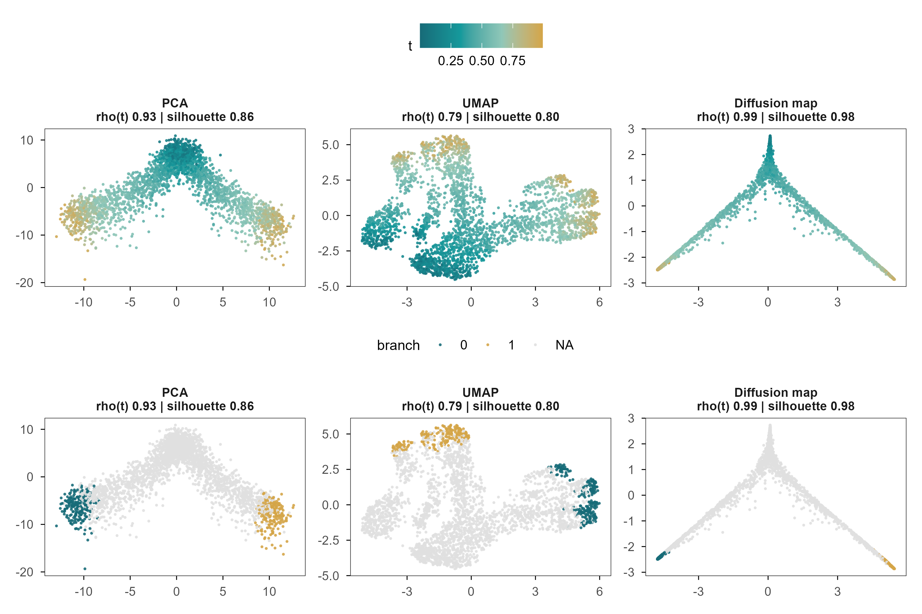
Figure 7: 图 5　PCA、UMAP 与 Diffusion Map 恢复的分化轨迹。颜色为真实分化进程 \(t\)；下排为同一嵌入按分支着色（仅 \(t>0.75\) 的细胞）。每个面板标题给出与 \(t\) 的 Spearman 相关和分支轮廓系数。 | Figure 5. The differentiation trajectory recovered by PCA, UMAP and diffusion maps. Colour is the true differentiation time \(t\); the lower row colours the same embeddings by branch (\(t>0.75\) cells only). Panel titles give the Spearman correlation with \(t\) and the branch silhouette.

三个面板都呈现出 Y 形分叉，但它们对同一条轨迹的表达并不相同。与 \(t\) 的相关：PCA 0.93，UMAP 0.79，Diffusion Map 0.99。在这个模拟里，PCA 已经很接近最优——因为我们的分化程序本来就是近似可加的。这说明「非线性方法更好」不是普遍规律，而是取决于流形是否真的弯曲。

All three panels show a Y-shaped bifurcation, but they express the trajectory differently. Correlation with \(t\): PCA 0.93, UMAP 0.79, diffusion maps 0.99. In this simulation PCA is already close to optimal, because the differentiation programmes were built to be approximately additive. Nonlinear methods are not universally better; it depends on whether the manifold is actually curved.

分支分离度则是另一回事。真实的分支轮廓系数是 0.68，三个方法分别给出 0.86、0.80、0.98——都被放大了，Diffusion Map 放大了约 1.4 倍。任何在二维图上「看起来分得很开」的两个分支，其真实差异都要打上折扣。

Branch separation is another matter. The true silhouette is 0.68; the three methods give 0.86, 0.80 and 0.98 — all inflated, diffusion maps by about 1.4-fold. Any two branches that look far apart in a 2-D plot are, in reality, closer than they appear.

5.4 伪时间不是时间 / Pseudotime is not time

Diffusion map 的特征值按「图上的尺度」排序，而不是按生物学排序。在我们这个系统里，第一个非平凡扩散分量与 \(t\) 几乎无关（相关 0.062），它跟踪的是分支；真正跟随 \(t\) 的是第二个分量（相关 0.985）。换句话说，如果你把 DC1 直接当作伪时间，你会得到分支，而不是时间。

The eigenvalues of a diffusion map are ordered by graph scale, not by biology. In our system the first non-trivial diffusion component is almost uncorrelated with \(t\) (0.062) and tracks the branch instead; the second component is the one that follows \(t\) (0.985). In other words, if you take DC1 as pseudotime you get the branch, not the time.

伪时间还有一个更根本的问题：它只是沿某条推断出来的路径的序号，与真实的日历时间、甚至与细胞的实际分裂次数都不是一回事。我们只能保证「顺序大致正确」，不能保证「间隔成比例」。

Pseudotime has a deeper problem: it is only the index of a cell along an inferred path, not calendar time and not the number of divisions. We can hope the ordering is roughly right; we cannot assume the spacing is proportional.

6. Autoencoder 与 VAE：学习一个可生成的空间 / Autoencoders and VAEs: Learning a Generative Representation

PCA 的编码器是线性的，UMAP 没有解码器，Diffusion Map 没有参数化的生成规则。想要一个既能编码又能生成的空间，最直接的做法是训练一对神经网络。

PCA’s encoder is linear, UMAP has no decoder, and diffusion maps have no parametric generative rule. If we want a space that both encodes and generates, the direct approach is to train a pair of neural networks.

6.1 Autoencoder 的优化目标 / The autoencoder objective

\[ \min_{\theta,\phi}\; \frac{1}{N}\sum_{i=1}^{N}\big\lVert x_i - g_\phi(f_\theta(x_i))\big\rVert^2 \]

这几乎就是把 PCA 的目标换成了非线性函数类。差别是本质性的：只要有足够宽的隐层，\(f_\theta\) 可以把弯曲的流形「摊平」，而线性投影做不到。代价是，重构目标本身不包含任何关于「潜在维度应该有意义」的约束——它只要求信息不丢失。

This is essentially the PCA objective with a nonlinear function class. The difference is fundamental: with wide enough hidden layers \(f_\theta\) can flatten a curved manifold, which a linear projection cannot. The cost is that the reconstruction objective contains no constraint that the latent dimensions be meaningful — only that information is not lost.

6.2 VAE：给潜在空间加一个先验 / Adding a prior to the latent space

VAE 引入两个分布：编码器输出近似后验 \(q_\phi(z\mid x)\)，先验 \(p(z) = \mathcal{N}(0, I)\)，解码器给出似然 \(p_\theta(x\mid z)\)。边缘似然 \(\log p(x)\) 不可直接计算，于是最大化其下界：

A VAE introduces two distributions: the encoder outputs an approximate posterior \(q_\phi(z\mid x)\), the prior is \(p(z)=\mathcal{N}(0,I)\), and the decoder gives the likelihood \(p_\theta(x\mid z)\). The marginal likelihood \(\log p(x)\) is intractable, so we maximise a lower bound:

\[ \log p(x) \;\ge\; \mathbb{E}_{q_\phi(z\mid x)}\big[\log p_\theta(x\mid z)\big] \;-\; D_{\mathrm{KL}}\big(q_\phi(z\mid x)\,\Vert\,p(z)\big) \;=\; \mathcal{ELBO} \]

用重参数化 \(z = \mu + \sigma \odot \epsilon,\ \epsilon\sim\mathcal{N}(0,I)\) 就能对 \(\phi\) 求梯度。第一项要求「从 \(z\) 能重建 \(x\)」，第二项要求「后验不要离先验太远」。两者相互拉扯：只有第一项，模型会退化成普通 autoencoder，潜在空间被撕成互不相连的点；只有第二项，模型退化成先验，什么都重建不出来。

Reparameterising as \(z = \mu + \sigma\odot\epsilon\) with \(\epsilon\sim\mathcal{N}(0,I)\) makes the bound differentiable in \(\phi\). The first term asks that \(x\) be reconstructable from \(z\); the second keeps the posterior near the prior. They pull against each other: with only the first term the model degenerates into an autoencoder whose latent space is torn into disconnected points; with only the second it collapses to the prior and reconstructs nothing.

6.3 一个真实的失败：ELBO 的尺度 / A real failure: the scale of the ELBO

我们第一版实现里，重建项对基因取平均、\(\beta = 1\)。训练曲线几乎是平的，测试误差与「直接预测均值」相同，潜在变量与任何真实因子都不相关——后验完全塌缩。原因不是模型容量，而是尺度：1000 个基因的平均平方误差约 0.9，而 4 维的 KL 项可以轻松达到几十。重建项在数值上被 KL 压倒了。

In our first implementation the reconstruction term was averaged over genes with \(\beta=1\). The training curve was flat, the test error equalled predicting the mean, and no latent dimension correlated with any true factor — complete posterior collapse. The cause was not capacity but scale: the mean squared error over 1,000 genes is about 0.9, while a 4-dimensional KL term easily reaches tens. Numerically, KL overwhelmed reconstruction.

修正办法是对基因求和而不是取平均，使两项处于同一量级：

The fix is to sum over genes rather than average, putting the two terms on the same scale:

\[ \mathcal{L} = \sum_{g}\big(x_{ig} - \hat x_{ig}\big)^2 \;+\; \beta\sum_{j} D_{\mathrm{KL}}\big(q(z_j\mid x_i)\,\Vert\,\mathcal{N}(0,1)\big) \]

这不是「调参技巧」，而是 ELBO 本身的结构：似然是对所有观测维度的联合概率，KL 是对潜在维度的，二者天然不在一个量级上。任何跨数据集比较 \(\beta\) 的做法，如果不说明维度，都是没有意义的。

This is not a tuning trick; it is the structure of the ELBO: the likelihood is a joint probability over all observed dimensions, the KL over latent dimensions, and the two live on different scales by construction. Comparing \(\beta\) across datasets without stating the dimensions is meaningless.

6.4 训练结果 / Training results

arch <- tibble(
  layer = factor(c("input", "h1", "h2", "latent", "h2d", "h1d", "output"),
                 levels = c("input", "h1", "h2", "latent", "h2d", "h1d", "output")),
  x = 1:7, w = c(1000, 256, 64, 8, 64, 256, 1000)
)
pA <- ggplot(arch, aes(x, y = w / 2)) +
  geom_rect(aes(xmin = x - 0.34, xmax = x + 0.34, ymin = 0, ymax = w), fill = cell_pal[["teal"]],
            alpha = 0.18, colour = cell_pal[["deep"]], linewidth = 0.4) +
  geom_text(aes(label = w), size = 2.8, colour = cell_pal[["ink"]]) +
  geom_segment(data = tibble(x = 1:6, xend = 2:7), aes(x = x + 0.34, xend = xend - 0.34,
              y = 0, yend = 0), inherit.aes = FALSE,
              arrow = arrow(length = unit(1.6, "mm")), colour = cell_pal[["grey"]]) +
  scale_y_log10() + labs(x = NULL, y = "units (log)", title = "autoencoder / VAE trunk") +
  theme(axis.text.x = element_blank(), axis.ticks.x = element_blank())

hist <- e4$history |> filter(d == 4)
pB <- ggplot(hist, aes(epoch)) +
  geom_line(aes(y = train / 1000, colour = model, linetype = "train"), linewidth = 0.6) +
  geom_line(aes(y = val / 1000, colour = model, linetype = "validation"), linewidth = 0.5) +
  scale_colour_manual(values = c(AE = cell_pal[["deep"]], VAE = cell_pal[["gold"]]), name = NULL) +
  scale_linetype_manual(values = c(train = "solid", validation = "22"), name = NULL) +
  labs(x = "epoch", y = "loss / 1000 genes", title = "training curves (d = 4)")

mse <- bind_rows(
  tibble(model = "PCA", d = e4$pca$d, mse = e4$pca$test_mse),
  tibble(model = e4$nn$model, d = e4$nn$d, mse = e4$nn$test_mse)
)
pC <- ggplot(mse, aes(factor(d), mse, colour = model, shape = model, group = model)) +
  geom_hline(yintercept = 1, linetype = "22", colour = cell_pal[["grey"]]) +
  geom_line(linewidth = 0.5) + geom_point(size = 2) +
  scale_colour_manual(values = c(PCA = cell_pal[["grey"]], AE = cell_pal[["deep"]], VAE = cell_pal[["gold"]]), name = NULL) +
  scale_shape_manual(values = c(15, 17, 16), name = NULL) +
  coord_cartesian(ylim = c(0.88, 0.95)) +
  labs(x = "latent dimensions", y = "test MSE (standardised)", title = "reconstruction")

(pA + pB + pC) + plot_layout(widths = c(1.15, 1, 0.95))

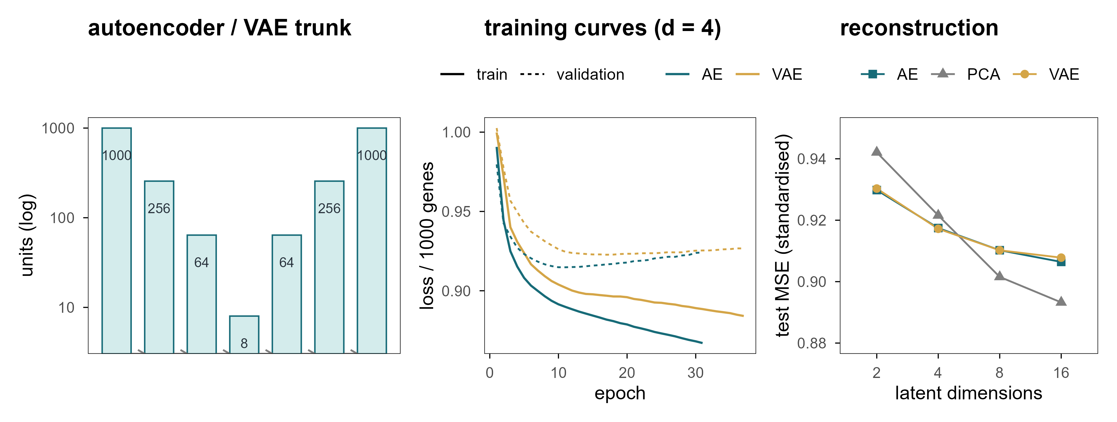
Figure 8: 图 6　(a) 网络结构：编码器与解码器共享同一个瓶颈。(b) 实际训练曲线（d = 4），点线为验证集。(c) 测试集重建误差随潜在维度的变化；灰色虚线是「直接预测均值」的误差。 | Figure 6. (a) Architecture: encoder and decoder share one bottleneck. (b) Actual training curves at d = 4, dotted line is validation. (c) Test reconstruction error versus latent width; the grey dashed line is the error of predicting the mean.

三点值得注意。第一，所有模型的测试误差都在 0.893–0.942 之间，而「直接预测均值」的误差是 1.0——它们只比什么都不做略好，这是因为数据里只有约 9% 的方差是信号。第二，维度增加带来的改善非常有限：从 2 维到 16 维，误差只从 0.930 降到 0.906。第三，非线性模型并没有显著胜过 PCA，因为在这个模拟里，线性结构已经足够。

Three things stand out. First, every model lands between 0.893 and 0.942, against 1.0 for predicting the mean — barely better than doing nothing, because only about 9% of the variance is signal. Second, extra dimensions buy very little: from 2 to 16 dimensions the AE error moves only from 0.930 to 0.906. Third, the nonlinear models do not clearly beat PCA, because the linear structure already suffices here.

6.5 概率潜在空间与插值 / A probabilistic latent space and interpolation

VAE 的价值不在于重构得更好，而在于它定义了整个空间的概率密度。这意味着我们可以从先验采样、可以在两点之间插值、可以问「这个区域有没有细胞」。我们在第 9 章会看到，这个能力既可以用来做实验设计，也可以用来制造幻觉。

The value of a VAE is not better reconstruction but that it defines a probability density over the whole space. That lets us sample from the prior, interpolate between points, and ask whether a region contains any cells at all. Chapter 9 shows that this ability can be used both for experimental design and for producing hallucinations.

为了处理计数数据，我们还训练了一个负二项解码器的版本：解码器输出期望表达 \(\mu\)，并以固定的文库大小偏移还原到计数尺度。

To handle counts we also trained a negative-binomial decoder: it outputs an expected expression \(\mu\) and maps back to the count scale with a fixed library-size offset.

\[ x_{ig}\sim\mathrm{NB}\!\left(\mu_{ig}\cdot\frac{L_i}{10^4},\ \theta_g\right), \qquad \log\mu_{ig} = h_\theta(z_i)_g \]

在留出细胞上，它的每基因负对数似然是 7.042，预测均值与观测计数的 Spearman 相关是 0.262。这两个数字说明它学到了整体的表达结构，但不说明它学到了因果机制。

On held-out cells its per-gene negative log-likelihood is 7.042 and the Spearman correlation between predicted mean and observed counts is 0.262. These numbers say it captured the overall expression structure; they say nothing about causal mechanism.

Z <- e5$Z
# pick the two latent dimensions that track t and the branch best
ct <- as.vector(abs(cor(Z, sim_truth$t, method = "spearman")))
cb <- as.vector(abs(cor(Z, sim_truth$s_branch, method = "spearman")))
i_t <- which.max(ct); i_b <- which.max(cb)
if (i_t == i_b) i_b <- setdiff(order(ct, decreasing = TRUE), i_t)[1]
tibble(z1 = Z[, i_b], z2 = Z[, i_t], t = sim_truth$t) |>
  ggplot(aes(z1, z2, colour = t)) +
  geom_point(size = 0.5, alpha = 0.8) +
  scale_colour_t(name = "t") +
  labs(x = sprintf("latent dimension %d (branch, rho = %.2f)", i_b, cb[i_b]),
       y = sprintf("latent dimension %d (time, rho = %.2f)", i_t, ct[i_t]))

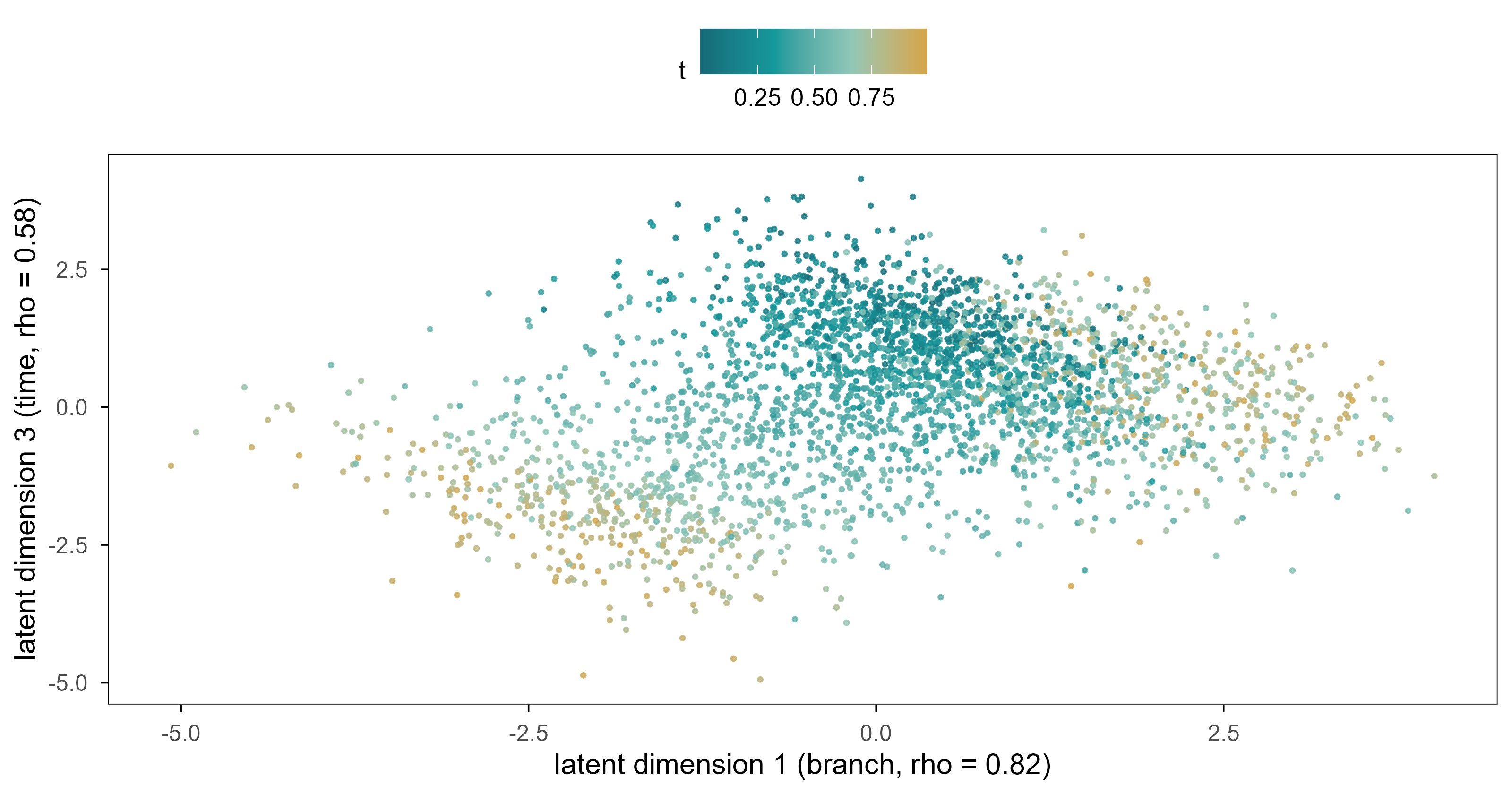
Figure 9: 图 7a　负二项 VAE 的四维潜在空间中分别跟踪分支与分化进程的两个维度。颜色为真实分化进程 \(t\)。 | Figure 7a. Two of the four latent dimensions of the negative-binomial VAE, tracking the branch and the differentiation time respectively. Colour is the true differentiation time \(t\).

高斯 VAE 的潜在空间里，有一个维度与分支高度相关（|ρ| = 0.82），但没有一个维度能干净地代表时间（最强也只有 0.58）——时间信息被分散在多个维度里。这与「潜在维度应当解耦」的直觉相反，而且在 VAE 里是常态：可逆线性变换不改变似然，所以模型没有任何动力把时间对齐到某一个轴上。

In the Gaussian VAE’s latent space one dimension tracks the branch strongly (|ρ| = 0.82), but no single dimension represents time cleanly (the best is 0.58); time is spread across several dimensions. This contradicts the intuition that latent dimensions should be disentangled, and it is the norm for VAEs: invertible linear maps leave the likelihood unchanged, so the model has no incentive to align time with any particular axis.

值得一提的是负二项版本：它的每基因负对数似然降到 7.04（高斯版本在标准化空间里的 MSE 为 0.917，两者不可直接比较，但趋势清楚：计数似然确实拟合得更好），然而它的潜在空间反而更差——与时间的相关只有 0.36，与激活状态的相关只有 0.17。更好的似然不等于更好的表征：计数似然把大部分容量花在了高表达基因的绝对值上，而状态信号藏在低表达基因的相对变化里。

The negative-binomial version is worth mentioning: its per-gene negative log-likelihood drops to 7.04 (not directly comparable to the Gaussian MSE of 0.917, but the direction is clear — the count likelihood fits better), yet its latent space is worse: correlation with time only 0.36 and with activation only 0.17. A better likelihood is not a better representation: the count likelihood spends most of its capacity on the absolute level of highly expressed genes, while the state signal lives in relative changes of lowly expressed ones.

alpha <- e5$paths$A_B_same_branch$alpha
pos <- (1 - alpha) %o% e5$Z[e5$cells[["A"]], ] + alpha %o% e5$Z[e5$cells[["B"]], ]
tibble(z1 = e5$Z[, i_b], z2 = e5$Z[, i_t]) |>
  plot_ly(x = ~z1, y = ~z2, type = "scattergl", mode = "markers",
          marker = list(size = 2.5, color = "rgba(160,170,175,0.35)"),
          name = "cells", hoverinfo = "skip") |>
  add_markers(x = pos[, i_b], y = pos[, i_t], mode = "markers",
              marker = list(size = 9, color = "#D4A547", line = list(color = "#28323C", width = 1)),
              name = "decoded",
              text = sprintf("alpha %.2f<br>branch A %.2f<br>branch B %.2f", alpha,
                             e5$paths$A_B_same_branch$modA, e5$paths$A_B_same_branch$modB),
              hoverinfo = "text", frame = alpha) |>
  animation_opts(frame = 120, transition = 0, redraw = FALSE) |>
  animation_slider(currentvalue = list(prefix = "alpha = ")) |>
  layout(xaxis = list(title = sprintf("dimension %d (branch)", i_b)),
         yaxis = list(title = sprintf("dimension %d (time)", i_t)),
         paper_bgcolor = "rgba(0,0,0,0)", plot_bgcolor = "rgba(0,0,0,0)")

Figure 10: 图 7b（交互）　沿潜在直线从细胞 A 走到细胞 B：滑动滑块改变 α，金色点给出解码后的位置（悬停可见两个分支模块的平均表达）。 | Figure 7b (interactive). Walking along the latent straight line from cell A to cell B: move the slider to change α; the gold point shows the decoded position, and hovering reveals the mean expression of the two branch modules.

这条直线上的每一点都能被解码成一套完整的表达谱。下一个问题自然是：这条直线上的中间状态，是否对应真实存在的细胞？第 9 章会给出一个明确的否定答案。

Every point on this line decodes to a full expression profile. The natural next question is whether the intermediate states correspond to real cells. Chapter 9 gives a clear negative answer.

7. 潜在空间中的距离有生物学意义吗？ / Does Distance in Latent Space Have Biological Meaning?

这是全文最容易出错、也最容易被忽略的一节。几乎每一篇单细胞论文都会写「细胞在 UMAP 上分成两群」，但「分成两群」到底对应什么，取决于你用的是哪个空间、哪种距离。

This is the section where it is easiest to go wrong, and where mistakes are most often ignored. Almost every single-cell paper says “cells separate into two groups on the UMAP”, but what “separate” means depends entirely on which space and which metric you used.

7.1 三种距离 / Three distances

• 基因空间的欧氏距离：直接反映表达谱差异，但被高维噪声严重稀释；两个生物学上相同的细胞，其欧氏距离可能远大于两个不同细胞。
  Euclidean distance in gene space: it directly measures expression differences, but is diluted by high-dimensional noise; two biologically identical cells can be farther apart than two different ones.
• 潜在空间的欧氏距离：坐标是我们自己选的，距离的尺度随坐标系变化；旋转、缩放、甚至任意可逆线性变换都不改变拟合优度。
  Euclidean distance in latent space: the coordinates are our choice, and the scale changes with them; rotation, scaling and any invertible linear map leave the fit unchanged.
• 沿流形的测地距离：最接近「细胞状态差多少」的直觉，但需要先有一个可靠的图，而图的构造本身又依赖尺度和近邻数。
  Geodesic distance along the manifold: closest to the intuition of “how different are these states”, but it requires a reliable graph, and building that graph depends on scale and neighbour count.

第二种距离的非唯一性可以用一句话说明：若 \(z = f(x)\) 与 \(\hat x = g(z)\) 是一对编码解码器，那么对任意可逆矩阵 \(A\)，\(z' = Az\) 配 \(g'(z') = g(A^{-1}z')\) 给出完全相同的重构。潜在空间的坐标从来没有被数据唯一确定过，我们看到的「轴」是优化算法与初始化共同选择的。

The non-uniqueness of the second kind can be stated in one line: if \(z=f(x)\) and \(\hat x = g(z)\) form an encoder-decoder pair, then for any invertible \(A\), \(z' = Az\) with \(g'(z') = g(A^{-1}z')\) gives exactly the same reconstruction. The coordinates of a latent space are never uniquely determined by the data; the axes we see are chosen jointly by the optimiser and the initialisation.

7.2 局部结构比全局距离更可靠 / Local structure survives better than global distance

在模拟数据里，前三个主成分与真实潜在空间的距离相关是 0.69，而 10 近邻重合率只有 0.12。两个数字的落差说明：嵌入能大致保持「谁离谁远」的排序，但保不住「谁是邻居」这种精细结构——而后者才是聚类、轨迹推断真正依赖的东西。

In the simulation, the distance correlation between the first three principal components and the true latent space is 0.69, while 10-nearest-neighbour overlap is only 0.12. The gap says: the embedding roughly preserves who is far from whom, but not the finer “who is next to whom” structure — and the latter is what clustering and trajectory inference actually rely on.

7.3 真实数据上的距离保真度 / Distance fidelity on real data

pA <- tibble(d_pc = e8$d_pca, d_um = e8$d_um) |>
  ggplot(aes(d_pc, d_um)) +
  geom_bin2d(bins = 60) +
  scale_fill_gradientn(colours = c("#F7FAFA", "#8FC7B8", "#159A9C", "#176B78"), name = "pairs") +
  labs(x = "distance in 30 PCs", y = "distance in UMAP",
       title = sprintf("PBMC3k, rho = %.2f", e8$dist_keep[["umap"]]))

cp <- aggregate(e8$pcs, by = list(label = e8$label), mean)
cu <- aggregate(e8$umap, by = list(label = e8$label), mean)
cent <- tibble(pc = as.vector(as.matrix(dist(cp[, -1]))),
               um = as.vector(as.matrix(dist(cu[, -1]))))
pB <- ggplot(cent, aes(pc, um)) +
  geom_abline(slope = 1, intercept = 0, linetype = "22", colour = cell_pal[["grey"]]) +
  geom_point(size = 2, colour = cell_pal[["deep"]]) +
  labs(x = "centroid distance in 30 PCs", y = "centroid distance in UMAP",
       title = sprintf("centroids, rho = %.2f", e8$centroid_keep[["umap"]]))

pC <- tibble(
  pair = c("10 nearest\nneighbours", "random\npairs"),
  d = c(e7$func[["resp_diff_neighbours"]], e7$func[["resp_diff_random"]])
) |>
  ggplot(aes(pair, d, fill = pair)) +
  geom_col(width = 0.55) +
  geom_text(aes(label = sprintf("%.2f", d)), vjust = -0.4, size = 3) +
  scale_fill_manual(values = c(cell_pal[["teal"]], cell_pal[["grey"]]), guide = "none") +
  coord_cartesian(ylim = c(0, 22.5)) +
  labs(x = NULL, y = "mean response difference",
       title = sprintf("rho(state, response) = %.2f", e7$func[["cor_state_response"]]))

(pA + pB + pC) + plot_layout(widths = c(1.1, 1, 0.8))

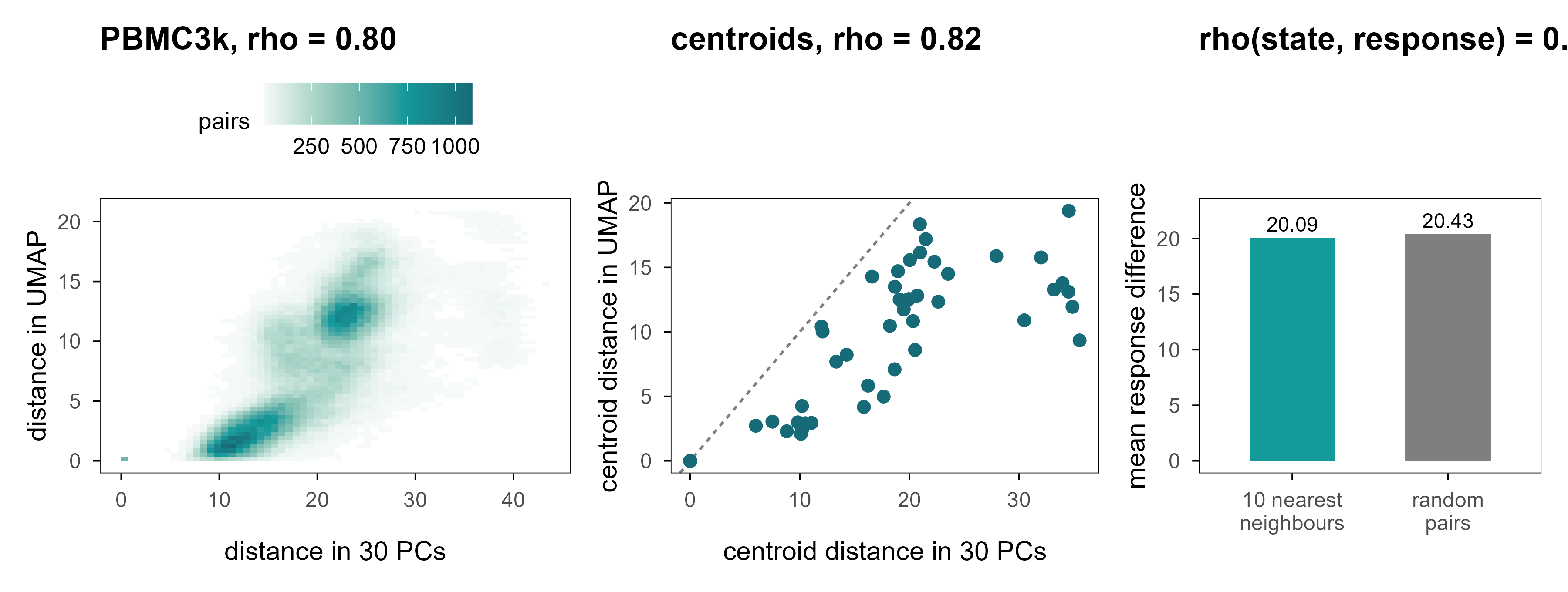
Figure 11: 图 8　潜在空间中的距离。(a) PBMC3k：500 个细胞两两之间的 30 维 PC 距离与 UMAP 二维距离（Spearman 相关见图内）。(b) 细胞类型质心之间的距离：横轴为 PC 空间，纵轴为 UMAP 空间；虚线为 \(y=x\)。(c) 模拟数据中，表达空间 10 近邻之间的扰动响应差异，与随机细胞对的响应差异几乎相同。 | Figure 8. Distances in latent space. (a) PBMC3k: pairwise 30-PC distance versus 2-D UMAP distance for 500 cells. (b) Distances between cell-type centroids in PC space (x) and UMAP space (y); the dashed line is \(y=x\). (c) In the simulation, perturbation-response differences between expression-space neighbours are almost as large as between random cell pairs.

图 8a 的相关系数是 0.80：在 PBMC3k 上，UMAP 的二维距离与 30 维 PC 距离的排序相关其实不低。但图 8b 揭示了问题所在——距离的比值被压缩或拉伸了。PC 空间里最远与最近的两个细胞类型质心之比是 Inf，在 UMAP 里变成 Inf。排序可以保持，尺度不能。

Panel 8a gives 0.80: on PBMC3k the rank correlation between 2-D UMAP distance and 30-PC distance is in fact decent. Panel 8b shows where the problem lies — the ratios are compressed or stretched. The ratio between the farthest and nearest cell-type centroids is Inf in PC space and Inf in UMAP. Ranks survive; scale does not.

这就解释了文献里一个反复出现的问题：UMAP 图上两个簇「看起来隔得很远」，读者会下意识地把它读成「这两种细胞差异很大」，但那个距离是优化器为了让簇分开而付出的代价之一。

This explains a recurring problem in the literature: two clusters “look far apart” on a UMAP, and readers instinctively read that as “these two cell types are very different” — but that distance is one of the prices the optimiser pays to separate clusters.

7.4 表达相似不等于功能相似 / Expression similarity is not functional similarity

图 8c 是本节最重要的结果。在同一批细胞、同一种扰动下，我们计算了表达空间里 10 近邻之间的扰动响应差异，以及随机细胞对之间的差异：20.1 对 20.4，相差不到 2%。表达状态与响应之间的距离相关只有 0.09。

Panel 8c is the most important result of this section. Under the same perturbation, the mean response difference between 10-nearest neighbours in expression space is 20.1, against 20.4 for random pairs — less than 2% smaller. The rank correlation between state distance and response distance is only 0.09.

这意味着：「这两个细胞在图上挨着」不能推出「它们对同一个干预会做出相同反应」。这正是「表征」与「因果模型」之间的那道缝隙：前者只保证观测相似，后者要求干预一致。第 9 章会把这个缝隙摊开来看。

Which means: “these two cells sit next to each other on the plot” does not imply “they will respond the same way to the same intervention.” This is precisely the gap between a representation and a causal model: the former only guarantees observational similarity, the latter demands interventional agreement. Chapter 9 opens that gap up.

8. 跨组学的共同潜在空间 / A Shared Latent Space Across Omics

同一个细胞可以同时被测转录组和表面蛋白，但绝大多数实验只能测其中一种。于是出现了一个非常实际的问题：如果我的 RNA 数据和别人的蛋白数据来自不同细胞、不同批次，我能不能把它们放到同一个坐标里？

The same cell can be profiled for transcriptome and surface proteins, but most experiments measure only one. That raises a practical question: if my RNA data and someone else’s protein data come from different cells and different batches, can they be placed in one coordinate system?

8.1 为什么这不是一个平移问题 / Why this is not a translation problem

如果两种模态是同一个潜在状态的线性函数，即 \(x_{\mathrm{RNA}} = A z + \epsilon_1\)、\(x_{\mathrm{prot}} = B z + \epsilon_2\)，那么存在一个线性映射 \(T = AB^{-1}\) 把两者对应起来，问题有唯一解（在 \(A, B\) 满秩时）。但现实里至少有三件事破坏了这一点：非线性（饱和、阈值）、模态特异的技术因素（捕获效率、抗体亲和力）、以及没有任何配对样本。

If the two modalities were linear functions of the same latent state — \(x_{\mathrm{RNA}} = Az+\epsilon_1\), \(x_{\mathrm{prot}} = Bz+\epsilon_2\) — then a linear map \(T = AB^{-1}\) would relate them and, with \(A\) and \(B\) of full rank, the solution would be unique. At least three things break this: nonlinearity (saturation, thresholds), modality-specific technical factors (capture efficiency, antibody affinity), and the absence of any paired samples.

最后一点是致命的。没有配对，「对齐」就变成了一个只有分布约束、没有对应约束的问题，而分布约束一般不足以确定对应关系。

The last point is fatal. Without pairing, alignment becomes a problem with distributional constraints but no correspondence constraints, and distributional constraints generally do not pin down the correspondence.

8.2 实验 6：四种对齐策略与一个反例 / Experiment 6: four strategies and one counter-example

我们用一个共享潜在状态生成 RNA（1000 个基因）与蛋白（60 个标记）两个模态，两组细胞不重叠，另外保留 60 个「锚点」细胞在两个模态中都被测量（模拟分选或少量多组学样本）。任务是检索：给定一个蛋白细胞，找到状态相同的 RNA 细胞。

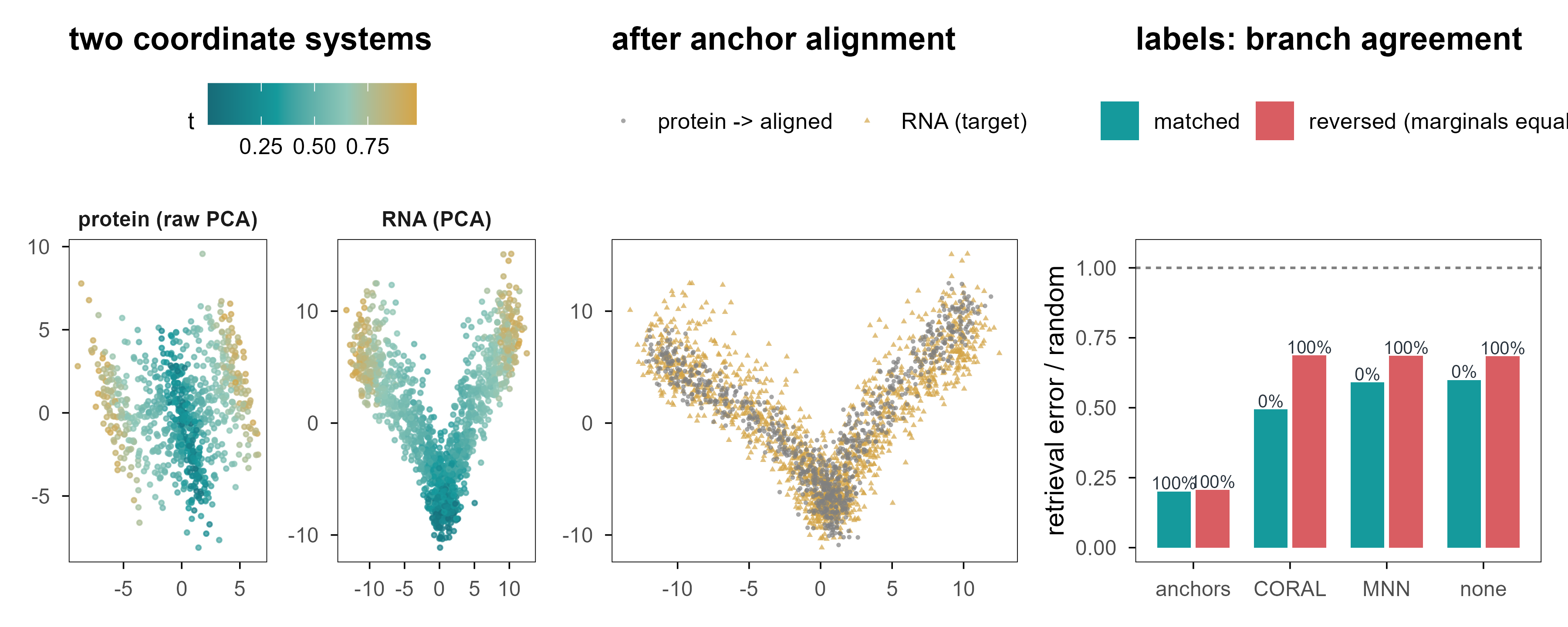
We generate RNA (1,000 genes) and protein (60 markers) from a shared latent state, with disjoint cell sets, plus 60 “anchor” cells measured in both modalities (mimicking sorting or a small multiome subset). The task is retrieval: given a protein cell, find the RNA cell in the same state.

emb <- e6$embeddings
dA <- bind_rows(
  tibble(space = "protein (raw PCA)", D1 = e6$p_pro[, 1], D2 = e6$p_pro[, 2], t = e6$truth_prot$t),
  tibble(space = "RNA (PCA)", D1 = e6$p_rna[, 1], D2 = e6$p_rna[, 2], t = e6$truth_rna$t)
)
pA <- ggplot(dA, aes(D1, D2, colour = t)) +
  geom_point(size = 0.6, alpha = 0.7) + scale_colour_t(name = "t") +
  facet_wrap(~ space, scales = "free", nrow = 1) + labs(x = NULL, y = NULL,
       title = "two coordinate systems")

dC <- bind_rows(
  tibble(set = "RNA (target)", D1 = e6$p_rna[, 1], D2 = e6$p_rna[, 2]),
  tibble(set = "protein -> aligned", D1 = emb[["matched anchors"]][, 1], D2 = emb[["matched anchors"]][, 2])
)
pB <- ggplot(dC, aes(D1, D2, colour = set, shape = set)) +
  geom_point(size = 0.55, alpha = 0.7) +
  scale_colour_manual(values = c(cell_pal[["grey"]], cell_pal[["gold"]]), name = NULL) +
  scale_shape_manual(values = c(16, 17), name = NULL) +
  labs(x = NULL, y = NULL, title = "after anchor alignment")

rr <- e6$res
rr$group <- ifelse(rr$scenario == "matched", "matched", "reversed (marginals equal)")
rr$agree_lab <- ifelse(is.na(rr$branch_agree), "", sprintf("%.0f%%", 100 * rr$branch_agree))
pC <- ggplot(rr, aes(method, dt_ratio, fill = group)) +
  geom_col(position = position_dodge(width = 0.8), width = 0.7) +
  geom_text(aes(label = agree_lab, y = dt_ratio + 0.03), position = position_dodge(width = 0.8),
            size = 2.6, colour = cell_pal[["ink"]]) +
  scale_fill_manual(values = c(cell_pal[["teal"]], cell_pal[["red"]]), name = NULL) +
  geom_hline(yintercept = 1, linetype = "22", colour = cell_pal[["grey"]]) +
  coord_cartesian(ylim = c(0, 1.05)) +
  labs(x = NULL, y = "retrieval error / random",
       title = "labels: branch agreement")

(pA + pB + pC) + plot_layout(widths = c(1.15, 1, 1))

Figure 12: 图 9　两个组学，一个潜在空间？(a) 蛋白模态的 PCA 空间（颜色为真实分化进程）与 RNA 模态的 PCA 空间不是同一个坐标系。(b) 用 60 个锚点细胞拟合线性映射后，蛋白细胞（金色）被放进 RNA 空间。(c) 四种方法的检索误差与分支一致性；右侧一组是「边际分布相同、生物学相反」的反例。 | Figure 9. Two modalities, one latent space? (a) The protein PCA space and the RNA PCA space are different coordinate systems. (b) After fitting a linear map on 60 anchor cells, protein cells (gold) land in RNA space. (c) Retrieval error and branch agreement for four methods; the right-hand group is the counter-example where marginals match but the biology is reversed.

rr <- e6$res
rr$branch_agree <- ifelse(is.na(rr$branch_agree), "—", sprintf("%.0f%%", 100 * rr$branch_agree))
knitr::kable(
  data.frame(
    `情景 / scenario` = ifelse(rr$scenario == "matched", "对齐 / matched", "反例 / reversed"),
    `方法 / method` = rr$method,
    `|Δt| / 随机` = sprintf("%.2f", rr$dt_ratio),
    `分支一致 / branch agreement` = rr$branch_agree,
    `MMD` = sprintf("%.3f", rr$mmd),
    check.names = FALSE
  ),
  caption = "非配对对齐的检索性能。 | Retrieval performance of unpaired alignment."
)

Table 6: 非配对对齐的检索性能。 | Retrieval performance of unpaired alignment.

情景 / scenario	方法 / method	|Δt| / 随机	分支一致 / branch agreement	MMD
对齐 / matched	none	0.60	0%	0.172
对齐 / matched	anchors	0.20	100%	0.005
对齐 / matched	CORAL	0.49	0%	0.019
对齐 / matched	MNN	0.59	0%	0.173
反例 / reversed	none	0.68	100%	0.187
反例 / reversed	anchors	0.21	100%	0.004
反例 / reversed	CORAL	0.69	100%	0.041
反例 / reversed	MNN	0.69	100%	0.183

四个结论：

Four conclusions:

1. 锚点最有效，而且答案稳定。 60 个配对细胞（占目标模态样本的 7%）把检索误差降到随机的 0.20，分支一致性 100%；把同一个流程用在反例上，结果几乎不变（0.21 与 100%）。
   Anchors work best and give stable answers. 60 paired cells (7% of the target modality) reduce retrieval error to 0.20 of random with 100% branch agreement; on the counter-example the same pipeline gives 0.21 and 100%.
2. 分布匹配能对齐形状，却把方向搞反了。 CORAL 把 MMD 从 0.172 压到 0.019——分布几乎完全重合——但检索误差仍有随机的 0.49，分支一致性 0%：它把 A 分支的细胞匹配到了 B 分支。
   Distribution matching aligns shape and inverts orientation. CORAL pushes MMD from 0.172 to 0.019 — the distributions nearly coincide — yet retrieval error stays at 0.49 of random with 0% branch agreement: it matches branch-A cells to branch-B cells.
3. 朴素 MNN 几乎没用。 在没有尺度归一化的情况下，互相最近邻的配对准确率很低，检索误差仍有随机的 0.59。
   Naive MNN barely helps. Without scale normalisation mutual-nearest-neighbour pairing is inaccurate and retrieval error remains 0.59 of random.
4. 反例暴露了符号的不确定性。 把蛋白模态的分支方向反转（边际分布完全不变）之后，CORAL 的分支一致性从 0% 变成 100%——同一个算法，在两个边际分布完全相同的世界里给出了完全相反的答案，而它在两个世界里的 MMD 都低于 0.041。一个输出会随任意符号约定翻转的方法，不能用来给细胞指定身份。
   The counter-example exposes sign indeterminacy. Flip the protein branch direction (marginals unchanged) and CORAL’s branch agreement moves from 0% to 100% — the same algorithm gives opposite answers in two worlds with identical marginal distributions, while its MMD stays below 0.041 in both. A method whose output flips with an arbitrary sign convention cannot assign biological identity.

这个实验的意义不只是「CORAL 不好」。它说明：在没有配对样本的情况下，「对齐」这个说法本身就是不完备的——你需要额外的结构假设（锚点、已知的对应细胞类型、共享的调控模块），而不同的假设会给出不同的、彼此不相容的对齐结果。

The point is not that CORAL is bad. It is that without paired samples the very notion of “alignment” is under-specified: you need additional structural assumptions (anchors, known matched cell types, shared regulatory modules), and different assumptions yield different, mutually incompatible alignments.

9. 在潜在空间中移动，可以改变细胞吗？ / Can We Change a Cell by Moving Through Latent Space?

这是全文的转折点。前面所有内容都关于「如何描述细胞现在的位置」；从这里开始，我们问「能不能把它移到别的位置」。这两件事在数学上看起来只差一步（在潜在空间里加一个向量），在科学上却隔着一整个因果推断。

This is the turning point. Everything so far has been about describing where a cell is; from here we ask whether we can move it somewhere else. Mathematically the two look one step apart (add a vector in latent space); scientifically they are separated by an entire theory of causal inference.

9.1 插值：几何上的直线，生物学的弯路 / Interpolation: a straight line in geometry, a detour in biology

最简单的「移动」是在两个细胞之间插值：

The simplest move is interpolation between two cells:

\[ z(\alpha) = (1-\alpha) z_A + \alpha z_B, \qquad \hat x(\alpha) = g_\phi\big(z(\alpha)\big) \]

每一步都可以解码成一套完整的表达谱，看起来非常像「细胞在分化」。但这里有两个陷阱：第一，直线只保证在坐标上连续，不保证在数据流形上连续；第二，即使落在流形上，也不保证这个中间状态是生物学上可实现的。

Every step decodes to a full expression profile and looks very much like differentiation. But there are two traps. First, the straight line is continuous in coordinates, not necessarily on the data manifold. Second, even if it lands on the manifold, the intermediate state need not be biologically realisable.

zz <- e5$Z
ct5 <- as.vector(abs(cor(zz, e5$truth$t, method = "spearman")))
cb5 <- as.vector(abs(cor(zz, e5$truth$s_branch, method = "spearman")))
jt <- which.max(ct5); jb <- which.max(cb5)
if (jt == jb) jb <- setdiff(order(ct5, decreasing = TRUE), jt)[1]
A <- e5$cells[["A"]]; B <- e5$cells[["B"]]; C <- e5$cells[["C"]]
pA <- ggplot(tibble(z1 = zz[, jb], z2 = zz[, jt], t = e5$truth$t), aes(z1, z2, colour = t)) +
  geom_point(size = 0.4, alpha = 0.6) +
  scale_colour_t(name = "t") +
  annotate("segment", x = zz[A, jb], y = zz[A, jt], xend = zz[B, jb], yend = zz[B, jt],
           colour = cell_pal[["deep"]], linewidth = 0.8, arrow = arrow(length = unit(2, "mm"))) +
  annotate("segment", x = zz[A, jb], y = zz[A, jt], xend = zz[C, jb], yend = zz[C, jt],
           colour = cell_pal[["red"]], linewidth = 0.8, linetype = "22",
           arrow = arrow(length = unit(2, "mm"))) +
  annotate("text", x = zz[A, jb], y = zz[A, jt], label = "A", size = 3.2, hjust = 1.2) +
  annotate("text", x = zz[B, jb], y = zz[B, jt], label = "B", size = 3.2, hjust = -0.2) +
  annotate("text", x = zz[C, jb], y = zz[C, jt], label = "C", size = 3.2, hjust = -0.2) +
  labs(x = sprintf("latent dim %d", jb), y = sprintf("latent dim %d", jt),
       title = "two paths")

px <- e5$paths$A_C_cross_branch
real_df <- tibble(t = e5$truth$t, contrast = e5$real_modA - e5$real_modB,
                  branch = factor(e5$truth$b)) |>
  filter(t > 0.1)
path_df <- bind_rows(
  tibble(t = e5$adm_pca$t, contrast = e5$adm_pca$contrast, decoder = "4-PC"),
  tibble(t = e5$adm_vae$t, contrast = e5$adm_vae$contrast, decoder = "VAE")
)
pB <- ggplot(real_df, aes(t, contrast)) +
  geom_ribbon(data = e5$band_grid, aes(x = t, ymin = lo, ymax = hi),
              inherit.aes = FALSE, fill = cell_pal[["mist"]], colour = cell_pal[["grey"]],
              linewidth = 0.3) +
  geom_hline(yintercept = 0, colour = cell_pal[["grey"]], linewidth = 0.3) +
  geom_point(aes(colour = branch), size = 0.5, alpha = 0.35) +
  geom_line(data = path_df, aes(group = decoder, linetype = decoder),
            colour = cell_pal[["red"]], linewidth = 0.9) +
  scale_colour_manual(values = c(cell_pal[["deep"]], cell_pal[["gold"]]), name = "branch") +
  scale_linetype_manual(values = c(`4-PC` = "solid", VAE = "22"), name = NULL) +
  labs(x = "differentiation time t", y = "branch A - branch B",
       title = "the 4-PC path runs ahead")

outside <- function(ad) ifelse(ad$contrast < ad$lo, ad$contrast - ad$lo,
                               ifelse(ad$contrast > ad$hi, ad$contrast - ad$hi, 0))
res_df <- tibble(
  t = c(e5$adm_pca$t, e5$adm_vae$t),
  res = c(outside(e5$adm_pca), outside(e5$adm_vae)),
  decoder = rep(c("4-PC", "VAE"), each = length(e5$adm_pca$t))
)
pC <- ggplot(res_df, aes(t, res)) +
  geom_hline(yintercept = 0, colour = cell_pal[["grey"]], linewidth = 0.4) +
  geom_line(aes(colour = decoder, linetype = decoder), linewidth = 0.8) +
  scale_colour_manual(values = c(cell_pal[["red"]], cell_pal[["deep"]]), name = NULL) +
  scale_linetype_manual(values = c(`4-PC` = "solid", VAE = "22"), name = NULL) +
  labs(x = "differentiation time t", y = "outside band",
       title = "overshoot") +
  theme(legend.position = "none")

(pA + pB + pC) + plot_layout(widths = c(1.15, 1.15, 0.85))

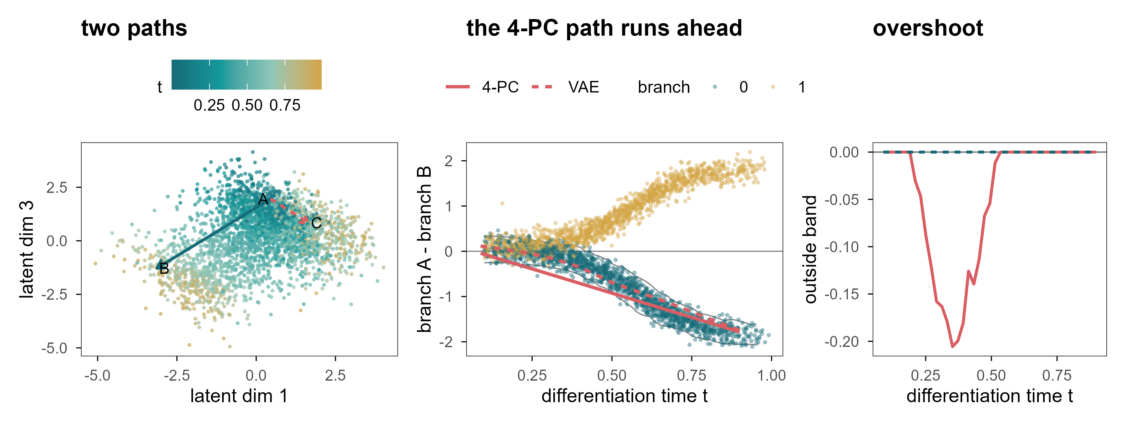
Figure 13: 图 10　最短直线不等于生物学路径。(a) VAE 潜在空间中的两条插值路径：A→B 在同一分支内，A→C 跨分支。(b) 真实细胞的「A 模块减 B 模块」对比随 \(t\) 的变化（点为真实细胞，颜色为分支）；灰带是同一时刻、目标分支真实细胞的 5–95% 区间。红色为插值路径（实线 4 维 PCA 解码器，点线 VAE 解码器）：两条路径最终都到达目标分支，但 4-PC 路径在中间段提前冲出灰带。(c) 两条路径偏离灰带（即真实细胞 5–95% 区间）的距离：VAE 全程为 0，4-PC 在中间段出现明显偏离。 | Figure 10. The shortest line is not a biological path. (a) Two interpolation paths in the VAE latent space: A→B within a branch, A→C across branches. (b) The branch-A-minus-branch-B contrast against \(t\) for real cells (points, coloured by branch); the grey ribbon is the 5–95% range of real cells at the same time in the target branch. Red lines are the interpolated paths (solid: 4-PC decoder, dotted: VAE). Both paths arrive at the correct branch, but the 4-PC path overshoots the ribbon in the middle. (c) Distance from every point of the path to the admissible band (the 5–95% range of real cells): the VAE stays at zero throughout, the 4-PC path departs from it in the middle.

图 10b 给出一个比「偏离流形」更微妙的失败。真实细胞在 \(t \approx 0.6\) 之后分成两支：一支 A 高 B 低，一支相反，中间几乎是空的。两条插值路径最终都到达了正确的分支——4 维 PCA 解码器在终点给出 -1.78，同一时刻真实细胞的 5–95% 区间是 -2.05 到 -1.55。只看终点，插值完全成功。

Panel 10b shows a subtler failure than “leaving the manifold”. After \(t \approx 0.6\) real cells split into two arms - A high and B low, or the reverse - and the middle is almost empty. Both paths do arrive at the correct branch: the 4-PC decoder ends at -1.78, while real cells at the same time span -2.05 to -1.55. Judged only by its endpoint, the interpolation is a complete success.

问题出在中间。真实的分支承诺不是匀速的：\(w(t)\) 在 \(t \approx 0.6\) 附近快速上升，早期细胞几乎没有分支特征，晚期细胞几乎完全确定。而潜在空间里的直线让「承诺」随 \(\alpha\) 匀速增长。结果是路径在 \(t \in [0.25, 0.5]\) 这一段冲出了灰带——它描述的是一个「分化到一半、却已经表达终末分支程序」的细胞，而这样的细胞在 3,000 个真实细胞里一个也没有。整条路径上有 39% 的点落在区间之外，最大偏差 0.21。值得注意的是，VAE 路径反而全程落在灰带内——这说明「通过这项检验」同样不能证明轨迹是生物学的，它只是没有犯这一个特定的错误。

The problem lies in the middle. Real commitment is not uniform in time: \(w(t)\) rises steeply around \(t \approx 0.6\), so early cells carry almost no branch signature and late cells are almost fully determined. A straight line in latent space makes commitment grow linearly in \(\alpha\). The consequence is that over \(t \in [0.25, 0.5]\) the path leaves the ribbon: it describes a cell that is halfway through differentiation yet already expresses a terminal branch programme, and no such cell exists among the 3,000 real ones. 39% of the path falls outside the interval, with a maximum excursion of 0.21. Notably, the VAE path stays inside the ribbon throughout — which shows that passing this test does not prove a trajectory is biological; it merely fails to make this particular mistake.

图 10c 把这一偏离直接画出来：4-PC 路径在 \(t \approx 0.25\)–\(0.5\) 区间稳定地落在灰带下方，VAE 路径全程贴住零线。更麻烦的是，这些插值点并没有「悬空」——它们到最近真实细胞的平均距离只有 0.67 倍于真实细胞自身的平均近邻距离。也就是说，一个「分化到一半却已表达终末程序」的细胞就落在数据云中央，被真实细胞团团包围。这正是最危险的情形：一个明显离谱的生成结果会被立刻发现，而一个「看起来完全正常」的中间谱不会。

Panel 10c draws the excursion directly: the 4-PC path sits steadily below the ribbon between \(t \approx 0.25\) and \(0.5\), while the VAE path hugs zero throughout. What makes it worse is that none of these points is floating in space — their mean distance to the nearest real cell is only 0.67 times a real cell’s own nearest-neighbour distance. A cell that is halfway through differentiation yet already expressing a terminal programme therefore sits in the centre of the cloud, surrounded by real cells. That is the most dangerous case of all: an obviously absurd generation is caught immediately, whereas a perfectly plausible-looking intermediate profile is not.

9.2 外推比插值危险得多 / Extrapolation is far more dangerous than interpolation

插值至少还有两个端点约束。外推没有：把 \(z\) 推到数据分布之外，解码器仍然会给出一个「看起来正常」的表达谱，因为它是一个函数，定义域是整个 \(\mathbb{R}^4\)。生成模型不会告诉你「这里没有数据」，除非你显式地问它。

Interpolation at least has two endpoints as constraints. Extrapolation has none: push \(z\) outside the data distribution and the decoder still returns a plausible-looking profile, because it is a function defined on all of \(\mathbb{R}^4\). A generative model will not tell you “there is no data here” unless you ask explicitly.

9.3 扰动：从「移动一个点」到「改变一个机制」 / Perturbation: from moving a point to changing a mechanism

真正有生物学意义的「移动」来自干预：敲除一个基因、激活一条通路、加一个药物。我们模拟了三种扰动，它们的效应都依赖细胞状态：

A genuinely biological “move” comes from an intervention: knock out a gene, activate a pathway, add a drug. We simulated three perturbations whose effects all depend on cell state:

\[ \Delta_{ig}(u) = -\,a_u\, m_{u,g}\, h_u(t_i, a_i), \qquad h_{u_1} = 0.2 + 1.6t,\quad h_{u_2} = 1.6 - 2.4t,\quad h_{u_3} = 0.4 + 1.2t + a \]

注意 \(h_{u_2}\)：它在 \(t \approx 0.67\) 处改变符号。同一个基因敲除，在早期细胞里压低某个模块，在晚期细胞里却抬高它。这不是人为设置的刁难，而是真实存在的现象（例如同一个转录因子在不同细胞状态下结合不同的增强子）。

Note \(h_{u_2}\): it changes sign at \(t \approx 0.67\). The same knockout lowers a module in early cells and raises it in late cells. This is not a contrived trap; it happens in real systems, for instance when the same transcription factor binds different enhancers in different states.

我们比较三种预测策略：固定响应向量（忽略状态）、近邻平均（用状态相近的已观测细胞的平均响应）、以及带状态交互项的线性模型。

We compare three strategies: a fixed response vector (ignoring state), neighbour averaging (average response of observed cells with similar state), and a linear model with state-by-perturbation interactions.

pr <- e7$res
knitr::kable(
  data.frame(
    `情景 / scenario` = pr$scenario,
    `方法 / method` = pr$method,
    `cos` = sprintf("%.2f", pr$cos),
    `R²` = sprintf("%.2f", pr$r2),
    `幅度比 / magnitude` = sprintf("%.2f", pr$magnitude),
    check.names = FALSE
  ),
  caption = "状态依赖扰动的预测性能（留出细胞）。 | Prediction of state-dependent perturbation responses on held-out cells."
)

Table 7: 状态依赖扰动的预测性能（留出细胞）。 | Prediction of state-dependent perturbation responses on held-out cells.

情景 / scenario	方法 / method	cos	R²	幅度比 / magnitude
u1	fixed	0.58	0.30	0.60
u1	kNN	0.56	0.30	0.60
u1	interaction	0.58	0.32	0.59
u2	fixed	0.56	0.28	0.56
u2	kNN	0.54	0.27	0.60
u2	interaction	0.55	0.29	0.58
u3	fixed	0.70	0.44	0.70
u3	kNN	0.68	0.43	0.71
u3	interaction	0.69	0.44	0.70
u2 (late, extrapolation)	fixed	-0.29	-0.79	0.64
u2 (late, extrapolation)	kNN	-0.26	-0.48	0.47
u2 (late, extrapolation)	interaction	-0.03	-0.18	0.40
u4 (unseen)	interaction	-0.09	-0.17	0.24
u4 (unseen)	null (0)	0.00	-0.06	0.00

三个结果值得逐条读：

Three results deserve a close read:

• 在观测覆盖的范围内，三种方法差不多。 u1、u2、u3 的 cos 都在 0.54–0.70。这说明：当干预覆盖了状态空间、且效应平滑时，复杂模型并不带来多少额外收益。
  Within the observed range the three methods are similar: cos between 0.54 and 0.70. When the intervention covers the state space and the effect is smooth, the complex model buys little.
• 一旦离开覆盖范围，固定向量会给出错误的方向。 对 u2 的晚期细胞，固定向量的 cos 是 -0.29，即方向完全相反。近邻法也好不到哪里去（-0.26），因为它在早期细胞里找不到可用的邻居。
  Once outside the covered range, the fixed vector points the wrong way. For late u2 cells its cos is -0.29, i.e. the opposite direction. Neighbour averaging is no better (-0.26), because it cannot find usable neighbours among early cells.
• 交互模型只能外推一小段。 它在 u2 晚期上的 cos 是 -0.03，R² 仍然是负的：线性外推在符号变化点附近还可以，但幅度完全错了。对从未观测过的 u4，所有方法都失败（cos -0.09，R² -0.17）。
  The interaction model extrapolates a little: cos -0.03 on late u2 cells, but R² stays negative — linear extrapolation gets the sign roughly right near the crossing point and the magnitude completely wrong. For the never-observed u4 every method fails (cos -0.09, R² -0.17).

vf <- e7$vfield
# normalise arrow lengths so the direction is visible on the cell scale
sc <- 1.2 / max(sqrt(vf$dx^2 + vf$dy^2))
cell_df <- tibble(z1 = e7$Z[, 1], z2 = e7$Z[, 2], t = e7$truth$t)
p <- plot_ly()
for (k in seq_along(c("u1", "u2"))) {
  u <- c("u1", "u2")[k]
  d <- vf[vf$u == u, ]
  p <- p |> add_segments(
    data = d, x = ~z1, y = ~z2, xend = ~z1 + dx * sc, yend = ~z2 + dy * sc,
    line = list(color = if (k == 1) "#159A9C" else "#D95D62", width = 3),
    visible = (k == 1), name = u, showlegend = FALSE,
    inherit = FALSE)
}
p <- p |>
  add_markers(data = cell_df, x = ~z1, y = ~z2, marker = list(size = 2, color = "rgba(150,160,165,0.30)"),
              name = "cells", hoverinfo = "skip") |>
  layout(
    xaxis = list(title = "PC1 (branch)"), yaxis = list(title = "PC2 (time)"),
    paper_bgcolor = "rgba(0,0,0,0)", plot_bgcolor = "rgba(0,0,0,0)",
    updatemenus = list(list(
      type = "buttons", direction = "right", x = 0.5, xanchor = "center", y = 1.15,
      buttons = list(
        list(label = "u1 (late-acting)", method = "update",
             args = list(list(visible = c(TRUE, FALSE, TRUE)), list(title = "u1: effect grows with t"))),
        list(label = "u2 (sign flip)", method = "update",
             args = list(list(visible = c(FALSE, TRUE, TRUE)), list(title = "u2: effect flips sign at t ~ 0.67")))
      )
    )),
    title = "u1: effect grows with t")
p

Figure 14: 图 11（交互）　状态依赖的扰动向量场。背景为细胞的潜在状态（PC1–PC2），箭头为该状态下预测的响应方向；点击按钮切换扰动。注意 u2 的箭头随位置翻转。 | Figure 11 (interactive). The state-dependent perturbation vector field. The background shows latent states (PC1-PC2); arrows give the predicted response direction at that state. Use the buttons to switch perturbation. Note that the u2 arrows flip direction along the trajectory.

图 11 里最值得看的是 u2 的箭头：它沿着分化轴逐渐缩短、然后反向。任何「用一个统一的扰动向量描述某个基因的作用」的做法，都会在这个图上暴露出问题。

The arrows worth watching in Figure 11 are those for u2: they shorten along the differentiation axis and then reverse. Any approach that describes a gene’s effect with one global perturbation vector is exposed by this picture.

9.4 状态转移函数需要什么 / What a state-transition function would need

如果想更进一步，从「预测某个状态下的响应」到「预测状态如何随时间演化」，需要的是一个动力系统：

Going further — from “predict the response at a state” to “predict how the state evolves in time” — requires a dynamical system:

\[ z_{t+\Delta t} = F_\theta\big(z_t,\; u_t,\; \Delta t\big), \qquad \hat x_{t+\Delta t} = g_\phi\big(z_{t+\Delta t}\big) \]

这个式子里每一项都有代价。\(F_\theta\) 需要在有干预的时间序列上训练，而这类数据极少；\(\Delta t\) 在真实数据里往往不可观测（我们用伪时间代替，而伪时间不是时间）；\(g_\phi\) 需要能把潜在状态还原成可测量的观测，而这一步又会引入所有前文讨论过的误差。

Every term in this equation has a cost. \(F_\theta\) needs training on interventional time series, which are rare; \(\Delta t\) is usually unobservable in real data (we substitute pseudotime, which is not time); and \(g_\phi\) must map latent states back to measurable observations, reintroducing every error discussed above.

更根本的是，一个能在观测数据上完美拟合的 \(F_\theta\)，可以在多个机制上等价。观测上的差异不等于因果上的干预：把两个状态的差异写成 \(\Delta x = x_1 - x_0\)，这只告诉我们「它们不同」，不告诉我们「是什么让它们不同」。

More fundamentally, an \(F_\theta\) that fits observational data perfectly can be consistent with several mechanisms. Observational difference is not causal intervention: writing the difference between two states as \(\Delta x = x_1 - x_0\) tells us that they differ, not what makes them differ.

10. 从潜在空间到虚拟细胞 / From Latent Representations to Virtual Cells

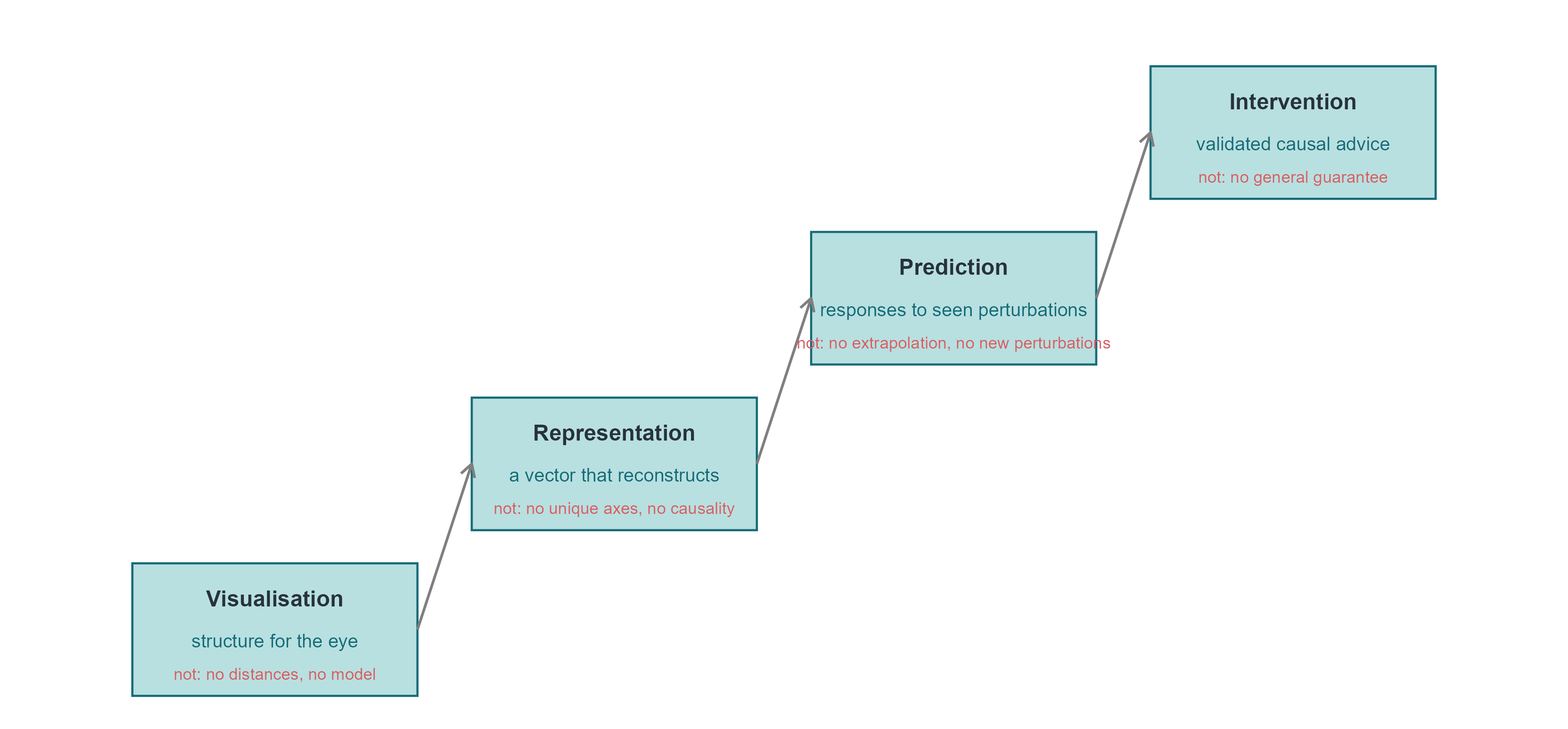
10.1 四个层次，四种承诺 / Four levels, four promises

「虚拟细胞」这个词被用来指代差别极大的东西。把它们分成四个层次，可以避免很多混淆：

The phrase “virtual cell” is used for very different things. Separating four levels avoids much confusion:

• 可视化（visualisation）：把细胞放到二维图上，帮助人眼发现结构。承诺很弱，也最容易兑现。
  Putting cells on a 2-D map so the eye can find structure. A weak promise, and the easiest to keep.
• 表征（representation）：得到一个可以重建、可以度量、可以迁移到下游任务的向量。承诺中等，需要独立的测试集。
  A vector that reconstructs, measures and transfers to downstream tasks. A medium promise, requiring independent test sets.
• 预测（prediction）：给定状态与干预，预测新的观测。承诺很强，需要干预数据与 OOD 检验。
  Given a state and an intervention, predict new observations. A strong promise, requiring interventional data and out-of-distribution tests.
• 干预（intervention）：给出的建议能被实验验证，并且能推广到未见过的细胞类型与扰动组合。承诺最强，目前几乎没有系统性的成功案例。
  Advice that survives experimental validation and generalises to unseen cell types and perturbation combinations. The strongest promise, with almost no systematic successes so far.

qA <- e2$metrics |> filter(key != "genes_direct")
pA <- ggplot(qA, aes(knn, r_t)) +
  geom_point(size = 2, colour = cell_pal[["teal"]]) +
  geom_smooth(method = "lm", se = FALSE, linewidth = 0.4, colour = cell_pal[["grey"]]) +
  labs(x = "10-NN preservation", y = "Spearman with t", title = "UMAP settings")

qB <- bind_rows(
  tibble(model = "AE", d = e4$nn$d[e4$nn$model == "AE"], mse = e4$nn$test_mse[e4$nn$model == "AE"],
         r_t = e4$nn$r_t[e4$nn$model == "AE"]),
  tibble(model = "VAE", d = e4$nn$d[e4$nn$model == "VAE"], mse = e4$nn$test_mse[e4$nn$model == "VAE"],
         r_t = e4$nn$r_t[e4$nn$model == "VAE"])
)
pB <- ggplot(qB, aes(mse, r_t, colour = model, label = d)) +
  geom_text(size = 3) +
  scale_colour_manual(values = c(AE = cell_pal[["deep"]], VAE = cell_pal[["gold"]]), name = NULL) +
  labs(x = "test reconstruction MSE", y = "Spearman with t", title = "AE / VAE (label = d)")

qC <- e7$res
pC <- ggplot(qC, aes(scenario, r2, fill = method)) +
  geom_col(position = position_dodge(width = 0.8), width = 0.7) +
  geom_hline(yintercept = 0, colour = cell_pal[["grey"]], linewidth = 0.3) +
  scale_fill_manual(values = c(fixed = cell_pal[["grey"]], kNN = cell_pal[["gold"]],
                               interaction = cell_pal[["teal"]], `null (0)` = "#DDDDDD"), name = NULL) +
  labs(x = NULL, y = "R² of predicted response", title = "perturbation prediction") +
  theme(axis.text.x = element_text(angle = 30, hjust = 1, size = rel(0.75)))

(pA + pB + pC) + plot_layout(widths = c(1, 1, 1.4))

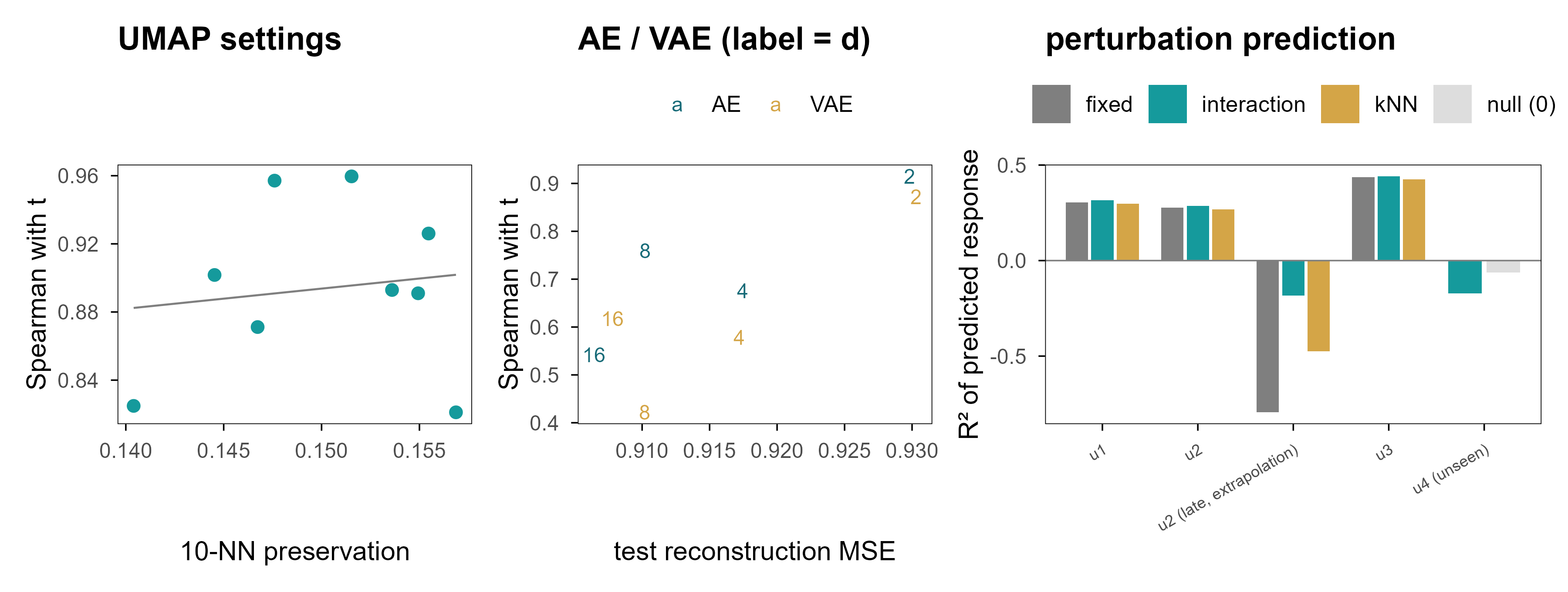
Figure 15: 图 12　「看起来好」与「预测得好」是两件不同的事。(a) 九组 UMAP 参数的近邻保持率与 \(t\) 恢复之间几乎没有关系。(b) 自编码器 / VAE 的重建误差越低，并不代表状态恢复越好：d = 2 的重建最差，却常常是 \(t\) 恢复最好的。(c) 扰动预测：在覆盖范围内 cos 很高，一旦外推 R² 立刻转负。 | Figure 12. Looking good and predicting well are different things. (a) Across nine UMAP settings there is almost no relation between neighbourhood preservation and recovery of \(t\). (b) Lower reconstruction error does not mean better state recovery: d = 2 reconstructs worst yet is often best for \(t\). (c) Perturbation prediction: cosine is high inside the covered range and R² turns negative as soon as we extrapolate.

三个面板说的是同一件事的三个方面：评价指标与目标能力之间没有必然联系。近邻保持率高的嵌入不一定恢复时间；重建误差低的模型不一定有可用的潜在坐标；在训练分布内 cos 很高的扰动模型，出了分布就失效。

The three panels say the same thing in three ways: the metric and the capability are not the same thing. An embedding with high neighbour preservation need not recover time; a model with low reconstruction error need not have usable latent coordinates; a perturbation model with high cosine inside the training distribution can fail immediately outside it.

10.2 真实数据上的同一件事 / The same story on real data

p1 <- tibble(U1 = e8$umap[, 1], U2 = e8$umap[, 2], label = e8$label) |>
  ggplot(aes(U1, U2, colour = label)) +
  geom_point(size = 0.35, alpha = 0.8) +
  scale_colour_manual(values = unname(cell_pal[c("teal", "deep", "gold", "red", "blue", "purple", "sky", "green", "orange", "grey")]),
                      name = NULL) +
  guides(colour = guide_legend(override.aes = list(size = 1.8), ncol = 1)) +
  labs(x = NULL, y = NULL, title = sprintf("%d cells, kNN purity %.2f", e8$n_cells, e8$purity)) +
  theme(legend.text = element_text(size = rel(0.6)),
        legend.key.height = unit(0.7, "lines"))

hm <- as.data.frame(e8$score) |>
  mutate(label = e8$label) |>
  pivot_longer(-label) |>
  group_by(label, name) |>
  summarise(v = mean(value), .groups = "drop")
p2 <- ggplot(hm, aes(name, label, fill = v)) +
  geom_tile(colour = "white", linewidth = 0.3) +
  geom_text(aes(label = sprintf("%.1f", v)), size = 1.9, colour = cell_pal[["ink"]]) +
  scale_fill_gradient2(low = "#176B78", mid = "#F7FAFA", high = "#D4A547", midpoint = 0, name = "score") +
  labs(x = NULL, y = NULL, title = "marker scores") +
  theme(axis.text.x = element_text(angle = 45, hjust = 1, size = rel(0.6)),
        axis.text.y = element_text(size = rel(0.6)),
        legend.key.height = unit(0.7, "lines"))

p3 <- ggplot(e8$qc, aes(n_gene)) +
  geom_histogram(bins = 40, fill = cell_pal[["deep"]], colour = NA) +
  labs(x = "genes detected", y = "cells", title = "QC")
(p1 + p2 + p3) + plot_layout(widths = c(1.1, 1.2, 0.7))

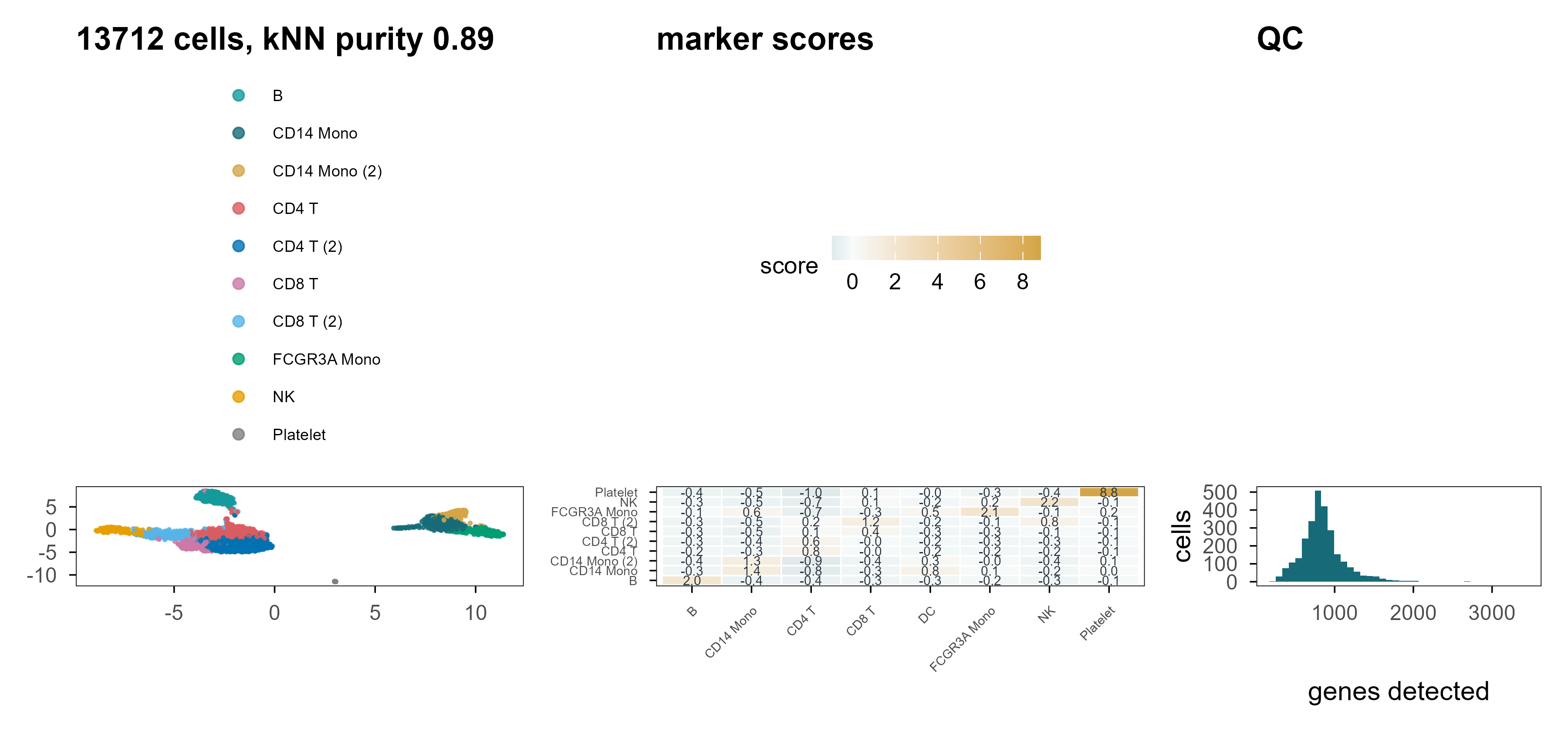
Figure 16: 图 13　PBMC3k 上的重复。(a) UMAP，颜色为 marker 打分 + k-means 得到的标签（不是金标准）。(b) 四个标记基因的表达。(c) 原始数据的 QC 分布。 | Figure 13. The same analysis on PBMC3k. (a) UMAP coloured by marker-score plus k-means labels (not a ground truth). (b) Expression of four marker genes. (c) QC distributions of the raw data.

在真实数据上，我们没有金标准，所以只能报告相对指标：kNN 标签纯度 0.89（这是在 PC 空间里用同一批标记算出来的，因此偏高）、PC1–10 解释 14.6% 的方差、UMAP 距离与 PC 距离的相关 0.80。这些数字能说明流程是自洽的，但不能说明标签是对的。这是真实数据与模拟数据最本质的差别：前者没有答案可以对照。

On real data we have no ground truth, so only relative metrics can be reported: kNN label purity 0.89 (computed in PC space with the same markers, hence optimistic), 14.6% of variance in PC1-10, and a UMAP-to-PC distance correlation of 0.80. These numbers show the pipeline is self-consistent; they do not show the labels are right. That is the essential difference between real and simulated data: the former offers nothing to check against.

10.3 下一代虚拟细胞需要什么 / What the next generation of virtual cells would need

把前九章的结论收拢，一个真正有用的细胞表征至少需要四件事，而目前的工具往往只提供其中一两件：

Pulling the previous nine chapters together, a genuinely useful cell representation needs at least four things, and current tools usually provide only one or two:

• 对干预稳定的坐标。 潜在维度应当在不同的扰动、批次、测序深度下保持含义不变。目前没有任何非监督方法能保证这一点。
  Coordinates stable under intervention. Latent dimensions should keep their meaning across perturbations, batches and depths. No unsupervised method currently guarantees this.
• 显式的不确定性。 一个细胞状态是一个分布，不是一个点。VAE 提供了这个框架，但标准高斯先验常常与真实的后验形状不匹配。
  Explicit uncertainty. A cell state is a distribution, not a point. VAEs provide the framework, but a standard Gaussian prior often mismatches the real posterior.
• 机制约束。 基因调控网络、通路成员关系、代谢约束，都可以作为先验注入模型，减少「看起来合理但不可能」的解。
  Mechanistic constraints. Regulatory networks, pathway membership and metabolic constraints can be injected as priors, ruling out solutions that look plausible but are impossible.
• 干预数据的规模。 这是最硬的一条限制。没有足够多、覆盖足够广的扰动实验，任何「虚拟细胞」都只是在观测分布内插值。
  Scale of interventional data. This is the hardest constraint. Without enough perturbation experiments covering enough of state space, any “virtual cell” is only interpolating inside the observed distribution.

lad <- tibble(
  level = factor(c("Visualisation", "Representation", "Prediction", "Intervention"),
                 levels = c("Visualisation", "Representation", "Prediction", "Intervention")),
  x = 1:4, y = c(0, 0.9, 1.8, 2.7),
  gives = c("structure for the eye", "a vector that reconstructs",
            "responses to seen perturbations", "validated causal advice"),
  not = c("no distances, no model", "no unique axes, no causality",
          "no extrapolation, no new perturbations", "no general guarantee")
)
ggplot(lad, aes(x, y)) +
  geom_rect(aes(xmin = x - 0.42, xmax = x + 0.42, ymin = y, ymax = y + 0.72),
            fill = cell_pal[["teal"]], alpha = 0.30,
            colour = cell_pal[["deep"]], linewidth = 0.4) +
  geom_text(aes(label = level), y = lad$y + 0.53, size = 3.1, fontface = "bold", colour = cell_pal[["ink"]]) +
  geom_text(aes(label = gives), y = lad$y + 0.30, size = 2.6, colour = cell_pal[["deep"]]) +
  geom_text(aes(label = paste("not:", not)), y = lad$y + 0.12, size = 2.3, colour = cell_pal[["red"]]) +
  annotate("segment", x = 1.42, xend = 1.58, y = 0.36, yend = 1.26,
           arrow = arrow(length = unit(2, "mm")), colour = cell_pal[["grey"]]) +
  annotate("segment", x = 2.42, xend = 2.58, y = 1.26, yend = 2.16,
           arrow = arrow(length = unit(2, "mm")), colour = cell_pal[["grey"]]) +
  annotate("segment", x = 3.42, xend = 3.58, y = 2.16, yend = 3.06,
           arrow = arrow(length = unit(2, "mm")), colour = cell_pal[["grey"]]) +
  coord_cartesian(xlim = c(0.4, 4.6), ylim = c(0, 3.6)) +
  theme_void()

Figure 17: 图 14　从嵌入到虚拟细胞：四个层次，以及每一层「不能保证」的东西。 | Figure 14. From embedding to virtual cell: four levels and what each of them does not guarantee.

10.4 回到开头的问题 / Back to the opening question

现在可以回答开头那个问题了：我们是在发现生物学的潜在空间，还是在构造一个恰好对模型有用的潜在空间？

We can now answer the question posed at the start: are we discovering the latent space of biology, or constructing a latent space that happens to be useful for our models?

这篇文章的证据支持一个分两半的答案。

The evidence in this article supports a two-part answer.

发现的部分是真的。 当数据里确实存在低维结构时（我们的模拟是这样，Swiss roll 是这样，PBMC 的细胞类型结构也是这样），不同的方法会收敛到相似的结构：PCA 的第二主成分、Diffusion Map 的第二个分量、VAE 的某一个潜在维度，都能跟踪同一条分化轴。这说明结构在数据里，不在算法里。

The discovery part is real. When low-dimensional structure genuinely exists — in our simulation, on the Swiss roll, and in the cell-type structure of PBMC — different methods converge on similar structure: PC2, the second diffusion component and one VAE latent dimension all track the same differentiation axis. The structure is in the data, not in the algorithm.

构造的部分也是真的。 距离的尺度、簇的分离度、潜在轴的旋转、插值路径上的中间状态，这些都不是数据给的，而是模型给的。我们在第 4、5、7、9 章分别看到了它们在多大程度上偏离真实。

The construction part is also real. The scale of distances, the separation of clusters, the rotation of latent axes, and the intermediate states along an interpolation path are not given by the data but by the model. Chapters 4, 5, 7 and 9 quantified how far each of them drifts from the truth.

这两件事并不矛盾。地图既反映地形，也反映绘制者的选择。问题不在于「有没有构造」，而在于是否把构造的部分明确标出来：报告路径到数据云的距离，报告簇间距离的失真程度，报告外推的失败区间。

The two are not contradictory. A map reflects both the terrain and the choices of its maker. The question is not whether construction happens, but whether the constructed part is labelled as such: report the distance from an interpolated path to the data cloud, report the distortion of inter-cluster distances, report the region where extrapolation fails.

我们的目标不仅是寻找细胞的低维表示，而是寻找能够保留理解、预测并最终干预生物系统所需信息的表征。

The goal is not merely to find a low-dimensional representation of cells, but to discover representations that preserve the information necessary to understand, predict, and eventually intervene in biological systems.

按这个标准衡量，本文展示的所有方法都还只是第一步。它们能帮助我们看，部分地帮助我们重建，很少能帮助我们预测，几乎不能帮助我们干预。而这条路的下一段，恐怕不在降维算法里，而在干预实验的设计里。

By that standard, every method shown here is only a first step. They help us see, partly help us reconstruct, rarely help us predict, and almost never help us intervene. The next stretch of the road probably lies not in dimensionality-reduction algorithms but in the design of perturbation experiments.

参考文献 / References

1. Jolliffe, I. T. & Cadima, J. (2016). Principal component analysis: a review and recent developments. Philosophical Transactions of the Royal Society A 374, 20150202. doi:10.1098/rsta.2015.0202
2. McInnes, L., Healy, J. & Melville, J. (2018). UMAP: Uniform Manifold Approximation and Projection for Dimension Reduction. arXiv 1802.03426. https://arxiv.org/abs/1802.03426
3. Becht, E., et al. (2019). Dimensionality reduction for visualizing single-cell data using UMAP. Nature Biotechnology 37, 38–44. doi:10.1038/nbt.4314
4. Coifman, R. R. & Lafon, S. (2006). Diffusion maps. Applied and Computational Harmonic Analysis 21, 5–30. doi:10.1016/j.acha.2006.04.006
5. Haghverdi, L., Buettner, F. & Theis, F. J. (2015). Diffusion maps for high-dimensional single-cell analysis of differentiation data. Bioinformatics 31, 2989–2998. doi:10.1093/bioinformatics/btv325
6. van der Maaten, L. & Hinton, G. (2008). Visualizing data using t-SNE. Journal of Machine Learning Research 9, 2579–2605. https://www.jmlr.org/papers/v9/vandermaaten08a.html
7. Tenenbaum, J. B., de Silva, V. & Langford, J. C. (2000). A global geometric framework for nonlinear dimensionality reduction. Science 290, 2319–2323. doi:10.1126/science.290.5500.2319
8. Kingma, D. P. & Welling, M. (2014). Auto-encoding variational Bayes. ICLR. https://arxiv.org/abs/1312.6114
9. Rezende, D. J., Mohamed, S. & Wierstra, D. (2014). Stochastic backpropagation and approximate inference in deep generative models. ICML. https://arxiv.org/abs/1401.4082
10. Lopez, R., Regier, J., Cole, M. B., Jordan, M. I. & Yosef, N. (2018). Deep generative modeling for single-cell transcriptomics. Nature Methods 15, 1053–1058. doi:10.1038/s41592-018-0229-2
11. Gayoso, A., et al. (2022). A Python library for probabilistic analysis of single-cell omics data. Nature Biotechnology 40, 163–166. doi:10.1038/s41587-021-01206-w
12. Argelaguet, R., et al. (2021). Computational principles and challenges in single-cell data integration. Nature Biotechnology 39, 1202–1215. doi:10.1038/s41587-021-00895-6
13. Korsunsky, I., et al. (2019). Fast, sensitive and accurate integration of single-cell data with Harmony. Nature Methods 16, 1289–1296. doi:10.1038/s41592-019-0619-0
14. Hie, B., Bryson, B. & Berger, B. (2019). Efficient integration of heterogeneous single-cell transcriptomes using Scanorama. Nature Biotechnology 37, 685–691. doi:10.1038/s41587-019-0113-3
15. Lotfollahi, M., Wolf, F. A. & Theis, F. J. (2019). scGen predicts single-cell perturbation responses. Nature Methods 16, 715–721. doi:10.1038/s41592-019-0494-8
16. Roohani, Y., Huang, K. & Leskovec, J. (2024). Predicting transcriptional outcomes of novel multigene perturbations with GEARS. Nature Biotechnology 42, 927–935. doi:10.1038/s41587-023-01905-6
17. Bunne, C., et al. (2023). Learning single-cell perturbation responses using neural optimal transport. Nature Methods 20, 1759–1768. doi:10.1038/s41592-023-01969-x
18. Norman, T. M., et al. (2019). Exploring genetic interaction manifolds constructed from rich single-cell phenotypes. Science 365, 786–793. doi:10.1126/science.aax4438
19. Replogle, J. M., et al. (2022). Mapping information-rich genotype-phenotype landscapes with genome-scale Perturb-seq. Cell 185, 2559–2575. doi:10.1016/j.cell.2022.05.013
20. Theodoris, C. V., et al. (2023). Transfer learning enables predictions in network biology. Nature 618, 616–624. doi:10.1038/s41586-023-06139-9
21. Levina, E. & Bickel, P. J. (2005). Maximum likelihood estimation of intrinsic dimension. NeurIPS 17. https://papers.nips.cc/paper/2004/hash/74934548253bcab8490ebd74afed7031-Abstract.html
22. Bengio, Y., Courville, A. & Vincent, P. (2013). Representation learning: a review and new perspectives. IEEE TPAMI 35, 1798–1828. doi:10.1109/TPAMI.2013.50
23. Hastie, T., Tibshirani, R. & Friedman, J. (2009). The Elements of Statistical Learning, 2nd ed. Springer. doi:10.1007/978-0-387-84858-7
24. Luecken, M. D. & Theis, F. J. (2019). Current best practices in single-cell RNA-seq analysis: a tutorial. Molecular Systems Biology 15, e8746. doi:10.15252/msb.20188746
25. 10x Genomics (2017). 3k PBMCs from a Healthy Donor (v1), filtered gene-barcode matrix. https://cf.10xgenomics.com/samples/cell-exp/1.1.0/pbmc3k/pbmc3k_filtered_gene_bc_matrices.tar.gz
26. R package uwot: https://github.com/jlmelville/uwot；R package torch: https://torch.mlverse.org/；Quarto: https://quarto.org/

引用说明：标有 DOI 的条目为已发表论文；Levina–Bickel 与 UMAP 原始论文以会议/预印本形式给出；最后一条为软件与数据来源。PBMC3k 数据集由 10x Genomics 公开发布，本文按其原始许可使用。

Citation note: entries with DOIs are published papers; the Levina–Bickel and UMAP papers are cited in their conference/preprint form; the final entry lists software and data sources. The PBMC3k dataset is publicly released by 10x Genomics and used under its original terms.