This article was researched and written by an AI system (Trae Agent) and has not been proofread line by line by a human. Every number below comes from an actual run of the scripts shipped with the post (experiments/E01–E10; the lattice animations are rendered by python/render_animations.py); code, parameters and .rds result files live in the post directory. All simulations are models, not measurements of real flocks, schools or tissues: they show which rules are sufficient for which macroscopic quantities, not how any particular organism works.
生成本文所用的提示词(压缩后) / Prompt used to generate this article (condensed)
写一篇中英双语长文《什么是涌现?》,要求:区分弱涌现与强涌现;给出局部更新规则、宏观变量、序参量、控制参数、相变的形式化定义;实现并用可复现的 R 实验展示元胞自动机(Game of Life、elementary CA)、Vicsek 群体运动(噪声与密度扫描、相图、3D、动画)、以及细胞通讯产生的空间图案(参数扫描、空间自相关);必须给出「视觉复杂 ≠ 涌现」的反例;讨论涌现与非线性、进化、信息的关系,以及对多智能体与「活模型」的启示。至少 12 张图,含动画、交互与 3D,红蓝配色,所有数字来自实际运行。
A long bilingual essay on emergence: weak vs strong emergence; a formal account of local update rules, macroscopic variables, order parameters, control parameters and phase transitions; reproducible R experiments on cellular automata (Game of Life, elementary CA), the Vicsek model (noise and density sweeps, phase diagram, 3-D, animation) and pattern formation by cell signalling (parameter scan, spatial autocorrelation); a counter-example showing that visual complexity is not emergence; links to nonlinearity, evolution and information, and to multi-agent and “living” models. At least twelve figures including animation, interaction and 3-D, red/blue palette, every number from an actual run.
1. 为什么「简单规则」会产生复杂世界? / Why Can Simple Rules Produce Complex Worlds?
A flock of starlings splits into ribbons at dusk and closes again; cells in a dish organise themselves into finger-like fronts within hours; slime moulds aggregate into a migrating slug when food runs out. Each bird, each cell, each amoeba does something small: it looks at a few neighbours and adjusts its heading or its state. No individual knows the shape of the whole.
That is the phenomenon this article is about. It has a familiar name — emergence — and the name tends to hide the interesting question. The interesting question is not “the whole is more than the sum of its parts”. It is: if the rules are this simple, why does macroscopic structure appear at all? When exactly does it appear? And once it does, what entitles us to say that it has?
1.1 微观与宏观之间没有同义词 / There is no dictionary between micro and macro
Between one bird and a flock, what is missing is not data but vocabulary. An individual’s state is position plus heading; the flock’s state is polarisation, density fluctuation, correlation length. There is no term-by-term dictionary between the two descriptions: no bird “has” a polarisation, just as no single water molecule “has” a temperature.
This is the technical core of everything that follows. Emergence is not a mysterious new substance; it is the appearance of variables that are defined only at a coarser scale. Whether such variables are trustworthy depends on three things: they can be measured independently, they change systematically with parameters, and they survive outside the model that produced them.
The ten sections follow one fixed route: definitions (Section 2), mathematics (Section 3), then three models that make the definitions run (Sections 4–6). Cellular automata show how rules generate structure; the Vicsek model shows how structure changes abruptly with a parameter; the cell-signalling model shows how structure becomes spatial pattern. Section 7 turns the three into a checklist of criteria, and gives a counter-example that looks complex but is not emergent. Sections 8–9 connect this to evolution, information and AI; Section 10 closes.
所有模拟都用 R 完成,参数、种子和结果文件随文附带。文中每一个数字都由内联代码从 .rds 中读出,不是手抄的。
All simulations are in R, with parameters, seeds and result files shipped alongside. Every number below is read from the .rds files by inline code rather than copied by hand.
2. 什么是涌现? / What Is Emergence?
2.1 一个可以操作的定义 / A definition that can be operated on
Let a system consist of \(N\) units, each updating by a local rule. A macroscopic quantity \(M\) is an emergent quantity if (i) it depends on the collective state rather than on any individual, (ii) it stabilises as \(N\) grows, and (iii) it cannot be read off any single unit’s state.
This turns “emergent” from an adjective into a noun phrase: not “this system is very emergent” but “this quantity of this system is emergent”. It demands three things at once: write down the formula for \(M\), measure how \(M\) behaves as \(N\) grows, and show that \(M\) cannot be reconstructed from individual-level information.
The philosophical literature usually separates two kinds. Weak emergence means the macroscopic property is in principle derivable from the microscopic rules, but only by simulation or computation — it cannot be predicted from a compact formula. Strong emergence means the macroscopic property cannot in principle be derived from the microscopic laws and requires new, irreducible laws.
This article uses only weak emergence, and goes one step further: only measurable weak emergence counts. The reason is practical. Strong emergence still has no widely accepted instance in the natural sciences; and weak emergence without measurement degenerates easily into “this picture looks nice”. Section 7 gives a concrete counter-example showing how large the gap can be.
2.3 「看起来复杂」不等于「存在涌现」 / “Looks complex” is not “is emergent”
A patterned image can arise in three completely different ways: (a) simple rules coupled to each other, producing organised macroscopic structure; (b) rules that simply hard-code the pattern; (c) no rules at all, just random numbers painted on a grid.
Case (c) is the one most often mistaken for emergence; case (b) is cheating; only (a) is what we mean. And (a) can only be separated from the others by quantitative indicators and parameter dependence: the macroscopic structure should change continuously or abruptly with a control parameter, should reproduce across random seeds, and should show longer spatial correlations than a random field. All three can be measured, and Section 7 measures them.
3. 如何从数学上描述涌现? / How Can Emergence Be Described Mathematically?
3.1 三层结构:个体、规则、宏观量 / Three layers: units, rules, macroscopic variables
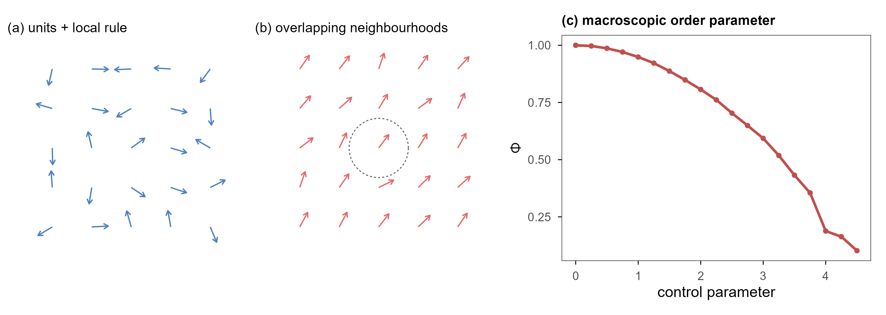
Figure 1: 图 1 从个体规则到宏观量的三层结构。(a) 每个个体只按自己的邻域更新;(b) 邻域重叠,于是信息沿局部链条传播;(c) 宏观量(这里是极化率)只在集体尺度上有定义,并随控制参数出现结构性改变。 | Figure 1. Three layers from individual rules to a macroscopic variable. (a) Each unit updates from its own neighbourhood; (b) neighbourhoods overlap, so information travels along local chains; (c) the macroscopic variable — here polarisation — exists only at the collective scale, and changes structure with a control parameter.
把系统写成三层,是所有后续讨论的基础。
Writing the system in three layers is the basis of everything that follows.
The first layer is the individual state. Unit \(i\) at time \(t\) has state \(x_i(t)\in\mathcal{X}\). In a cellular automaton \(x_i\in\{0,1\}\); in the Vicsek model \(x_i=(\mathbf{r}_i,\theta_i)\), position and heading.
The second layer is the local rule. Each unit looks only at its neighbourhood \(\mathcal{N}_i(t)\) (defined by distance or by the lattice) and updates through one shared function \(F\):
Here \(\theta\) is a set of global parameters — noise, density, threshold, diffusion. The crucial restriction is that\(F\) depends neither on \(i\) nor on \(N\). Every unit uses the same rule; no unit knows its own index in the system.
\(G\) must be symmetric (swapping the labels of any two units leaves the result unchanged); otherwise \(M\) would depend on labels rather than on the collective state.
3.2 序参量:把「有序」变成一个数 / Order parameters: turning “order” into a number
The most common macroscopic variable is the order parameter: a quantity that vanishes in the disordered phase and is non-zero in the ordered one. Polarisation in the Vicsek model is the cleanest example:
The geometry is direct: string the unit heading vectors head to tail and \(\Phi\) is the length of the resultant divided by \(N\). If all units point the same way, \(\Phi=1\); if headings are uniform on the circle, the resultant shrinks like \(1/\sqrt{N}\), so \(\Phi\to 0\). Note that \(1/\sqrt{N}\): a finite disordered system never sits exactly at zero, which is the origin of every “small systems look more ordered” effect later on.
3.3 控制参数与相变 / Control parameters and phase transitions
A control parameter is the knob we can turn in an experiment: noise \(\eta\), density \(\rho\), feed rate \(F\). If some macroscopic quantity changes structurally near a critical value of that knob, we call it a phase transition.
判据要写清楚,否则「相变」会变成对所有变化的统称。一个合格的相变陈述需要三件事:
The criterion must be stated explicitly, otherwise “phase transition” becomes a synonym for “change”. A defensible claim of a phase transition needs three things:
序参量:哪个量在变? Which quantity is changing?
控制参数:变的是哪个旋钮? Which knob is being turned?
极限行为:\(N\to\infty\) 时是否存在一个尖锐的临界点,还是仅仅是一个被有限尺寸抹平的过渡? Does a sharp critical point exist as\(N\to\infty\), or is it only a crossover smeared by finite size?
The third point is skipped most often and matters most. In a finite system any “jump” is smooth; a phase transition is the family of curves that get steeper as \(N\) grows. One way to test this is to compare \(\Phi(\eta)\) for several \(N\): only if the curves steepen with \(N\) and the steepening converges to a common \(\eta_c\) is there a transition.
对连续相变,还可以定义磁化率(极化率的涨落)作为辅助判据:
For a continuous transition one can also define a susceptibility (the fluctuation of the order parameter) as a second diagnostic:
\(\chi\) peaks near the critical point, and the location of the peak estimates \(\eta_c\). This article does not go that far (that would need more system sizes), but writing \(\chi\) down makes the point: “phase transition” has a mathematical test, it is not an impression from a picture.
Why does order disappear once noise passes some level? A one-line mean-field argument makes it clear. Let each unit’s heading equal the mean heading of its neighbours plus independent noise \(\xi\), and assume that the neighbour mean is approximately the global mean (this is the mean-field approximation: spatial correlations are ignored). Substituting into the definition of \(\Phi\) gives the self-consistency equation
This holds only if either \(\Phi=0\) (the disordered phase) or the mean cosine of the noise equals 1 (only possible at zero noise). Hence: mean field predicts a critical noise beyond which\(\Phi\) can only be zero. The argument ignores three things — spatial correlations, finite size, and the shape of the noise distribution — and those three determine the actual critical value and how sharp the transition is. Section 5 quantifies all three numerically.
One warning to finish the section: an order parameter describes structure, not function. A perfectly aligned flock of particles performs no task; a pattern that repairs itself might. So Section 7 asks three further questions beyond “is there an order parameter”: is the structure stable (does it recover after a perturbation), is it reproducible (does it survive a change of seed), and does it have a scale (is the correlation length far larger than the spacing between units)? Together these separate “a pattern” from “an organisation”.
Cellular automata (CA) are the cleanest instrument for testing the definition above. There are no continuous variables, no noise, no physics — only states, neighbourhoods and rules. If macroscopic structure appears even here, it cannot have been smuggled in.
4.1 定义 / The definition
一个二维 CA 由四件事确定:
A two-dimensional CA is fixed by four things:
网格:\(L\times L\) 的格点,本文取环面边界(上下、左右相接),以排除「边界效应」这个额外解释。 Lattice: an\(L\times L\) grid on a torus, so that “edge effects” cannot be an alternative explanation.
状态:每个格点 \(x_i\in\{0,1\}\)。 State:\(x_i\in\{0,1\}\) per site.
邻域:Conway 规则用 Moore 邻域,即 8 个相邻格点。 Neighbourhood: the Moore neighbourhood of 8 sites for Conway’s rule.
规则:一个把「当前状态 + 邻居状态」映射到「下一状态」的函数 \(F\)。 Rule: a function\(F\) from (own state, neighbour count) to the next state.
4.2 Game of Life:三条规则 / The Game of Life: three rules
Conway 的「生命游戏」把规则压到两行:
Conway’s Game of Life compresses the rule into two lines:
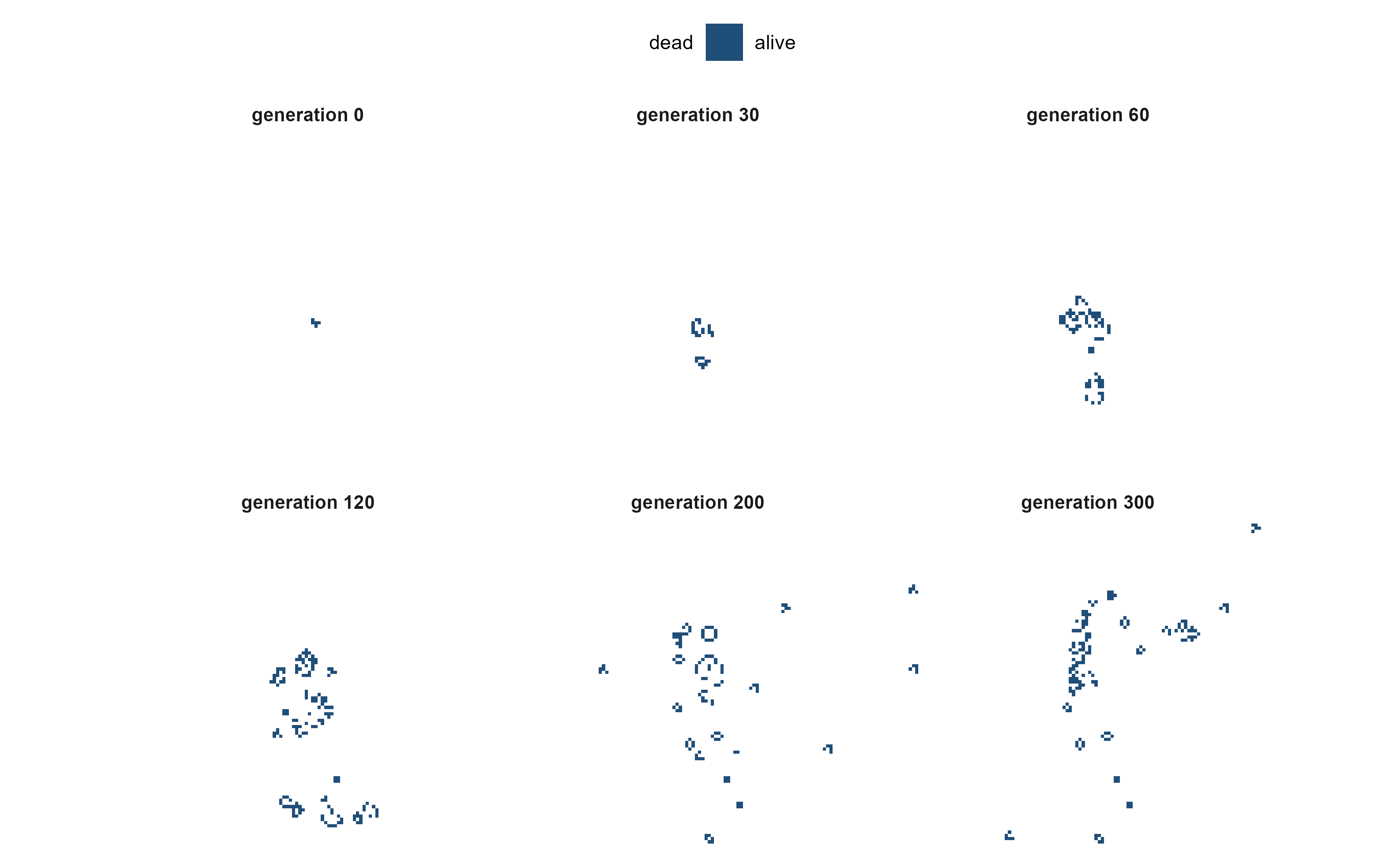
Birth needs exactly 3 neighbours, survival needs 2 or 3, everything else dies. There is no shape, no direction, no memory. Yet under these three rules one finds gliders (translating one cell diagonally every four generations), blinkers, blocks, and — starting from the five-cell R-pentomino — a chaotic expansion that lasts for more than a thousand generations.
Code
gol_long <-local({# crop all six frames to the same window, taken from the extent at the last# generation, so the growth of the object is visible and no cell is off-frame last <- gol$snaps[[length(gol$snaps)]] idx <-which(last >0, arr.ind =TRUE) r0 <-max(1, min(idx[, 1]) -4); r1 <-min(nrow(last), max(idx[, 1]) +4) c0 <-max(1, min(idx[, 2]) -4); c1 <-min(ncol(last), max(idx[, 2]) +4)do.call(rbind, lapply(seq_along(gol$snaps), function(k) { m <- gol$snaps[[k]][r0:r1, c0:c1] d <-expand.grid(x =seq_len(nrow(m)), y =seq_len(ncol(m))) d$alive <-as.vector(m) d$gen <- gol$gens[k] d }))})gol_long$gen <-factor(gol_long$gen, levels = gol$gens,labels =paste0("generation ", gol$gens))ggplot(gol_long, aes(x, y, fill =factor(alive))) +geom_raster() +scale_fill_manual(values =c(`0`="#FFFFFF", `1`= em_pal[["deep_blue"]]),labels =c("dead", "alive"), name =NULL) +coord_fixed(expand =FALSE) +facet_wrap(~gen, nrow =2) +theme(axis.text =element_blank(), axis.title =element_blank(),axis.ticks =element_blank(), panel.border =element_blank())
Figure 2: 图 2 R-pentomino 的六个时刻。初始只有 5 个活细胞,200 代之后系统仍在扩张;局部规则始终没有变。 | Figure 2. Six moments of the R-pentomino. It starts as five live cells and is still expanding after 200 generations; the local rule never changes.
What matters in Figure 2 is not the pattern but its extent: after 300 generations the live cells are still confined to a bounded region (sparse inside, but bounded), rather than filling the lattice uniformly. That region has no name and was designed by nobody; it is a product of three rules in time.
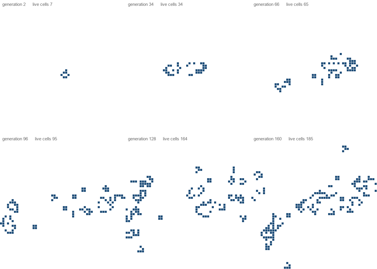
图 3 生命游戏的实时演化(每 2 代一帧),窗口跟随活细胞的外接框中心。 / Figure 3. The Game of Life in real time (one frame every two generations); the window follows the centre of the bounding box of the live cells.
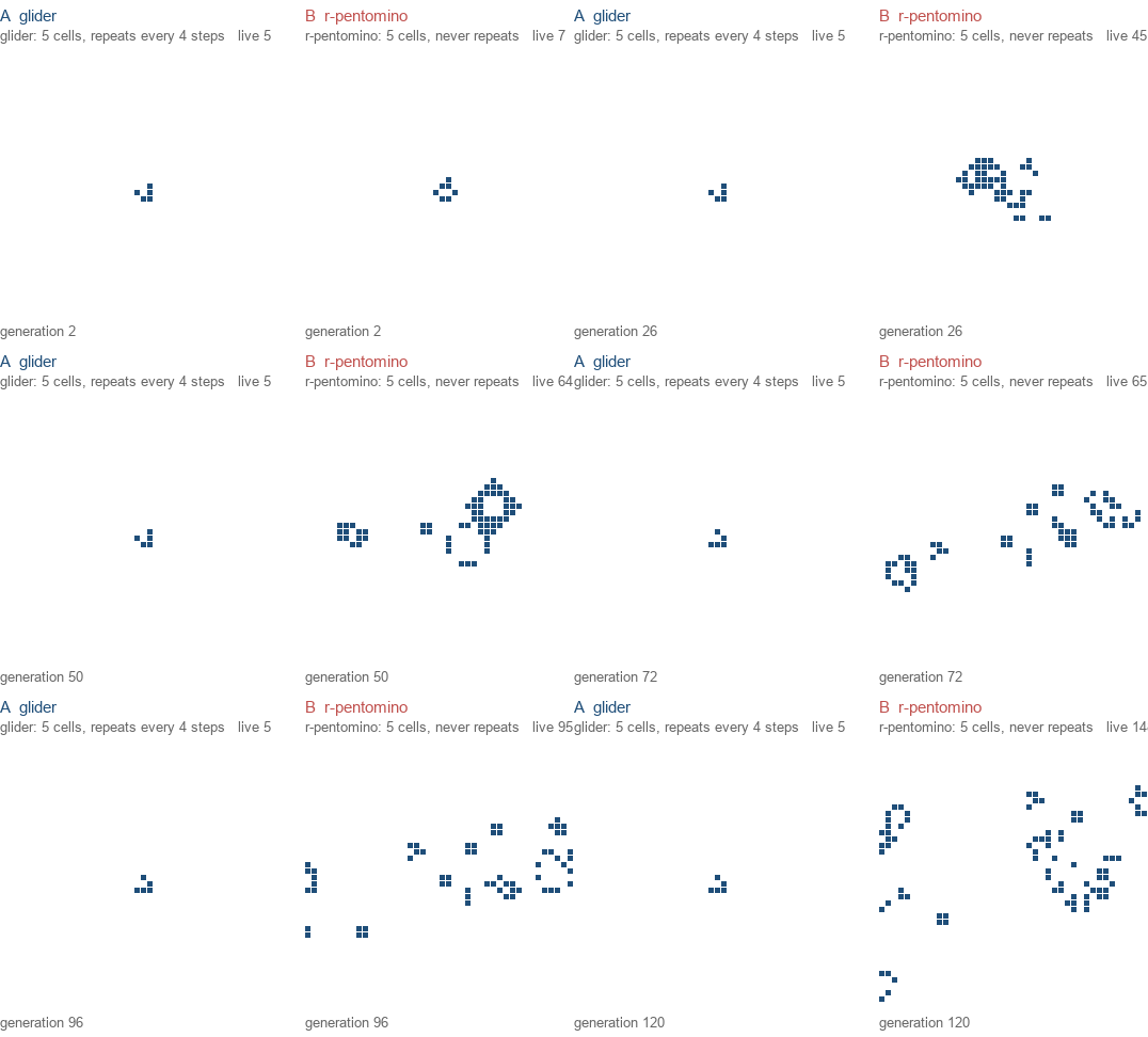
图 4 同一条规则,两种命运。A 是滑翔机:5 个细胞,每 4 代回到完全相同的形状,只是整体平移了一格;窗口跟着它走,所以画面上它几乎不动。B 是 R-pentomino:同样 5 个细胞,120 代之内从未重复自己。两边只有 5 个格子的排列不同。 / Figure 4. One rule, two fates. A is the glider: five cells that return to exactly the same shape every four generations, merely translated by one cell; the window follows it, so on screen it hardly moves. B is the r-pentomino: also five cells, which never repeats itself within 120 generations. The only difference between the two panels is the arrangement of five cells.
Side by side, the two animations make the phrase “simple rule” precise. Both start from five live cells under the same rule; the only difference is how the five cells are arranged: the left panel enters a period-4 cycle by generation four, the right panel sustains non-repetition for over a hundred generations. A simple rule does not imply simple behaviour, and complex behaviour does not imply a complex rule. This is the first empirical support for the definition in Section 2: there is no dictionary between micro and macro, because one and the same \(F\) produces both a period-4 cycle and non-repetition, while neither “period” nor “non-repetition” appears in \(F\).
4.3 一维基本元胞自动机:256 个世界 / Elementary CA: 256 possible worlds
Drop to one dimension and the rule space becomes small enough to enumerate. Each site sees only its two neighbours, so there are \(2^3=8\) possible neighbourhoods; a rule assigns an output to each, giving \(2^8=256\) rules numbered 0–255 (Wolfram encoding).
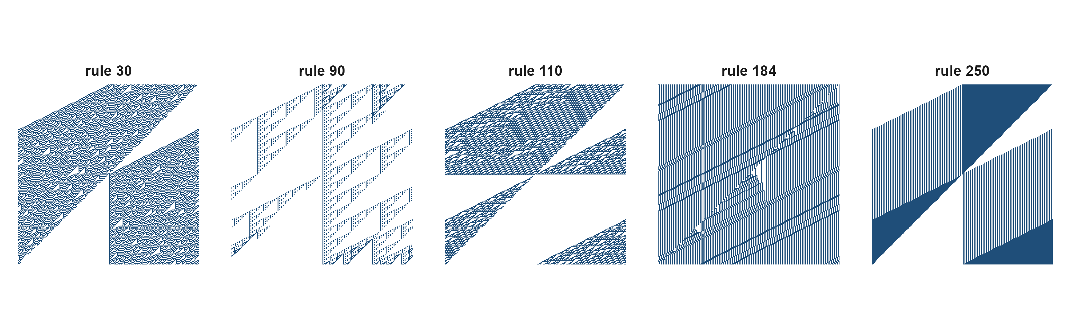
Figure 3: 图 5 五条规则。除 rule 184 外,初始条件都是中央一个活细胞(rule 184 用随机初始行,因为单个细胞无法产生「交通堵塞」)。横轴是空间,纵轴是时间(向下)。同一套「看邻居、查表」的机制,产生从规则条纹到混沌的五种世界。 | Figure 5. Five rules. Except for rule 184, the initial condition is a single live cell in the middle (rule 184 starts from a random row, because one cell cannot produce a traffic jam). Space is horizontal, time runs downwards. One mechanism — look at the neighbours, consult a table — produces five different worlds, from regular stripes to chaos.
Figure 5 contains at least three kinds of behaviour. Rule 90 produces a regular fractal triangle; rule 184 settles into stripes travelling to the left (a traffic-flow model); rules 30 and 110 both look “messy”, yet their computational status is completely different — rule 110 is Turing-complete, while the centre column of rule 30 is used as a random-number generator. “Looks messy” and “has structure” are different claims, and Section 7 puts numbers on that sentence.
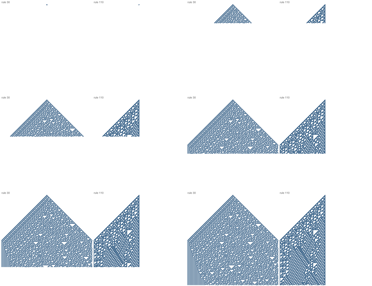
图 6 同一条规则逐代生长的过程(每 2 代一帧)。rule 30 的三角形保持完整的因果锥,内部却没有任何可预测的纹理;rule 110 的三角形一开始就分裂出斜向的「滑翔」结构,这些结构之后互相碰撞、湮灭、再生——图灵完备正来自这些碰撞。 / Figure 6. The same rule growing generation by generation (one frame every two generations). The rule 30 triangle keeps a clean causal cone but has no predictable texture inside; the rule 110 triangle immediately throws off diagonal glider-like structures that collide, annihilate and regenerate — the Turing completeness lives in those collisions.
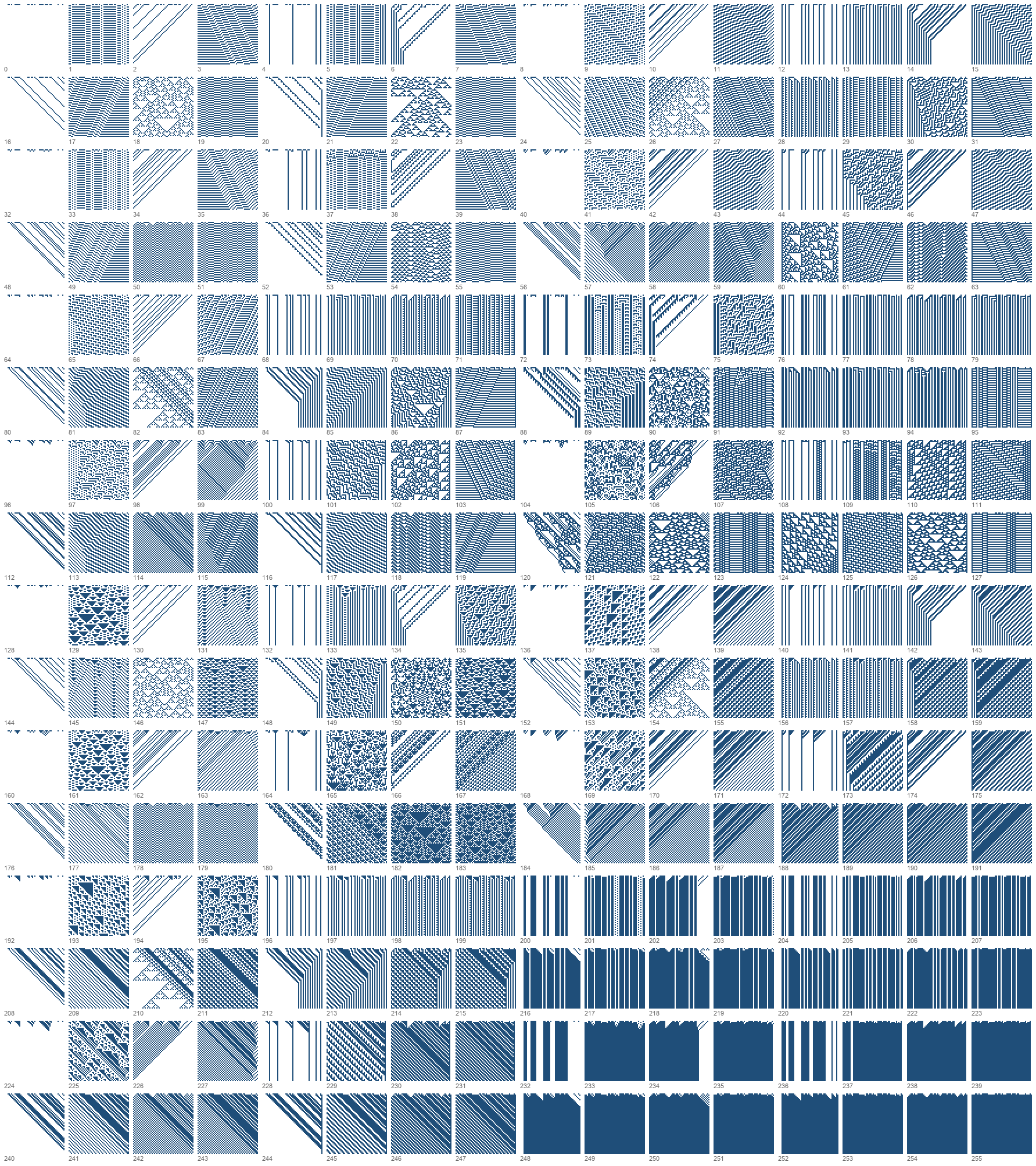
图 7 全部 256 条规则的全景(同一随机初始行,纵向为时间,可放大查看)。规则空间不是一条从「简单」到「复杂」的直线:有整片死寂(rule 0、rule 255),有规则的斜纹,有分形,也有局部沸腾的区块;而且编号相邻的规则行为并不相邻。 / Figure 7. All 256 rules from the same random initial row, time downwards (zoom in to read individual rules). The rule space is not a line from “simple” to “complex”: there are regions of total stillness (rules 0 and 255), regular diagonals, fractals, and patches that boil locally; neighbouring rule numbers do not have neighbouring behaviour.
The atlas is worth a pause, because it lays out the difference between rule space and behaviour space. The rule number is just a binary encoding: flip one of the eight output bits of rule 30 and you get rule 31, with entirely different behaviour; meanwhile two rules far apart in number can land in the same behavioural class. The number carries no behavioural information, so complexity cannot be inferred from the numbering — the rules have to be run and measured.
4.4 宏观量随时间怎么变? / What do the macroscopic variables do in time?
只有图案还不够。按第 3 节的定义,我们需要在每一代都计算宏观量,看它是否稳定、是否可复现。
A picture is not enough. Following Section 3, the macroscopic variables must be computed at every generation, to see whether they stabilise and whether they reproduce.
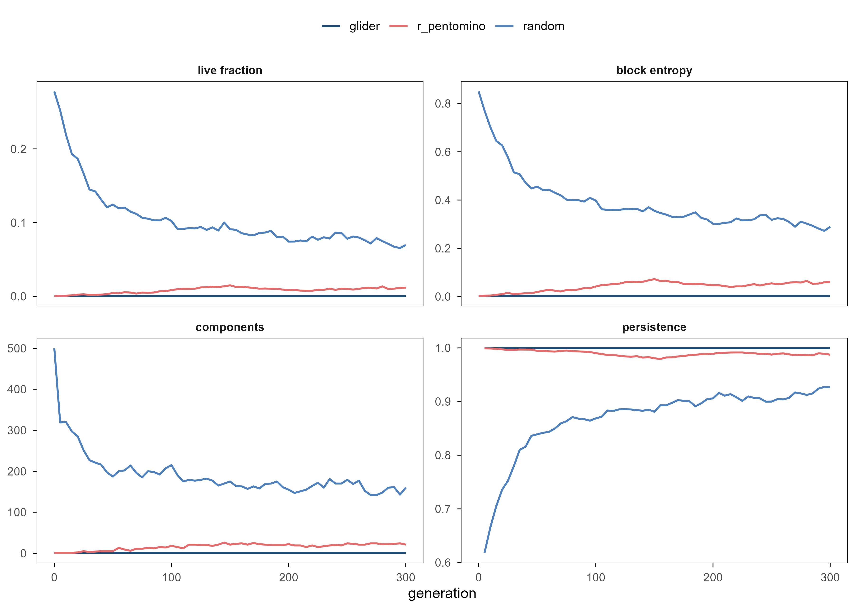
Figure 4: 图 8 三种初始条件下的四个宏观量。活细胞比例、块熵、连通块数量、相邻两帧的保持率。滑翔机在 300 代内保持单一连通块与近乎完全的帧间保持;随机汤则分裂成上百个小块并持续翻搅。 | Figure 8. Four macroscopic variables for three initial conditions: live fraction, block entropy, number of connected components, and frame-to-frame persistence. The glider keeps a single component and near-perfect persistence for 300 generations; the random soup fragments into hundreds of patches and keeps churning.
The four quantities divide the labour. Live fraction answers “how full”; block entropy answers “how unpredictable the local configuration is”; component count answers “how many pieces the pattern has broken into”; persistence answers “how stable the structure is”. Any one alone misleads: the entropy of the random soup falls from 0.85 to 0.29, but only because the lattice is emptying out, not because structure appeared.
把三行放在一起看,才有本文要的那种结论:
Only the three rows together give the conclusion this article is after:
The glider row is the cleanest example in the article. Its live fraction is only 0.03%, essentially nothing; yet it has exactly one connected component, the largest share is 1, and persistence is 0.999. In other words: 99.97% of the lattice is empty, and the thing occupying three cells is a persistent, mobile object that can be destroyed by collisions with other structures. No rule mentions a glider.
That is the standard shape of weak emergence: the glider can be derived from the rule (just run it), but not by a compact formula; at the macroscopic scale it is a stable entity, at the microscopic scale it is a set of cells flipping by rule. Whether it counts as strong emergence, the answer is no — it is fully determined by three rules and needs no new law.
The glider looks like an object, so the natural question is how robust it is. Flip each of the nine cells in its 3×3 bounding box in turn (alive to dead, dead to alive), run 40 more generations, and see whether it is still there.
The answer is 0 out of 9: not one single-cell flip leaves the glider unchanged. Of these, 4 die out entirely and the rest turn into some other still life or oscillator. So “the glider is a macroscopic object” and “the glider is stable” are two different claims: it is an emergent entity, but not a robust one.
The distinction matters in biology too. A cell type, an organ shape, an ecological equilibrium are all emergent entities; whether they recover after a perturbation depends on error-correcting mechanisms (feedback, redundancy, repair), not on their being emergent. The stability check in Section 7 exists precisely to hold that place.
5. 群体运动:Vicsek 模型与从无序到有序 / Collective Motion: The Vicsek Model and the Transition from Disorder to Order
元胞自动机有一个隐忧:它的宏观图案是静态的,而生命系统最显眼的能力是运动中的协调。鸟群没有中心控制器,鱼群在受惊时半秒内整体转向。Vicsek 模型(Vicsek et al., 1995)用最少的机制解释了这件事。
Cellular automata carry one worry: their macroscopic patterns are static, while the most conspicuous ability of living systems is coordination in motion. A flock has no central controller, and a school of fish can turn as a whole in half a second. The Vicsek model (Vicsek et al., 1995) explains this with the least possible machinery.
5.1 三条规则 / Three rules
\(N\) 个粒子在边长 \(L\) 的环面上以恒定速率 \(v\) 运动。每一步:
\(N\) particles move at constant speed \(v\) on a torus of side \(L\). At each step:
找到半径 \(r\) 内的所有邻居; find every neighbour within radius \(r\);
把自己的朝向角改成邻居平均朝向,再加上一个均匀噪声 \(\xi_i\sim U(-\eta/2,\eta/2)\); replace your heading by the neighbours’ mean heading, plus uniform noise \(\xi_i\sim U(-\eta/2,\eta/2)\);
沿新朝向前进 \(v\,\Delta t\)。 move forward by \(v\,\Delta t\) along the new heading.
Note the \(\arg\sum e^{i\theta}\) form: it handles the wrap-around of angles automatically (\(0\) and \(2\pi\) are the same heading), and it averages directions rather than numbers — the two differ completely across \(\pm\pi\), and this is the most common implementation error in this class of models.
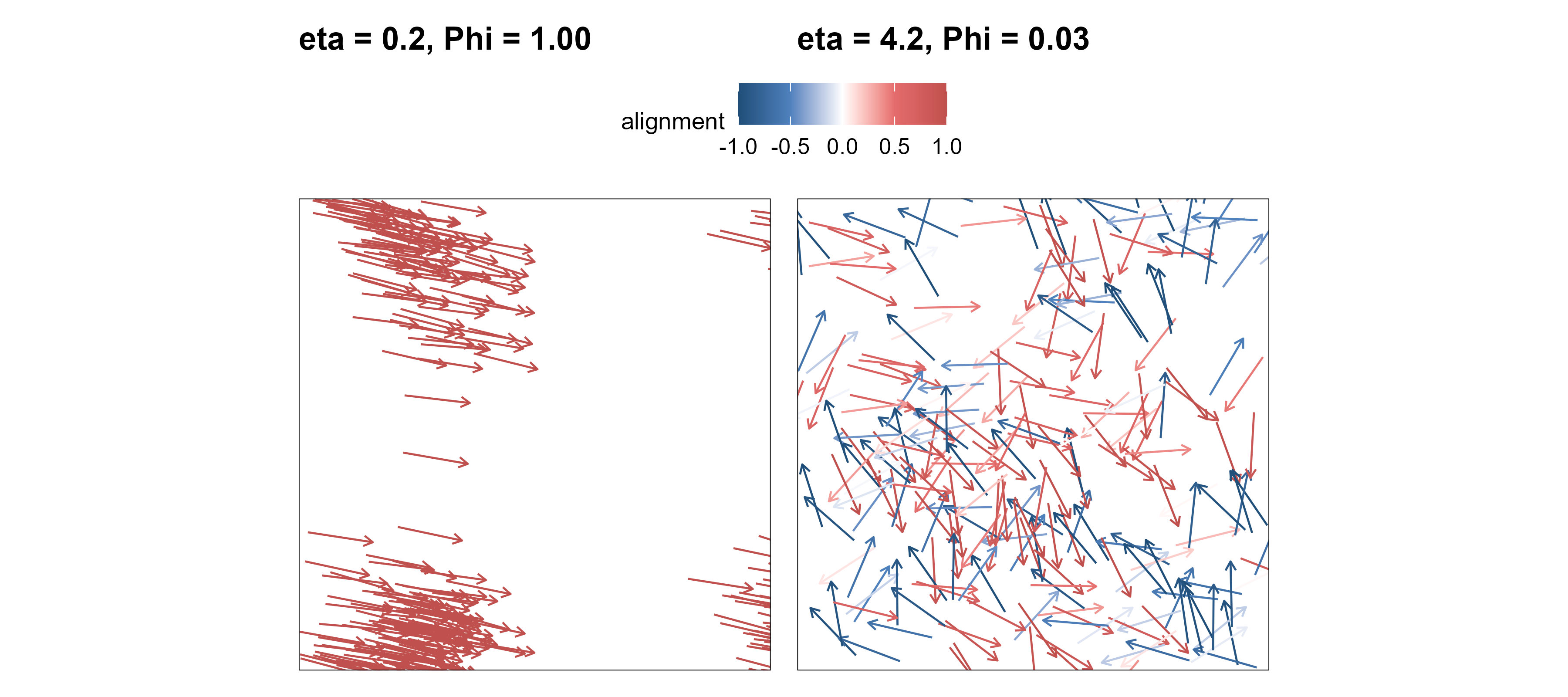
Figure 5: 图 9 同一模型、同一密度、同一速度,只改噪声。左:噪声 \(\eta=0.2\),粒子在几十步内对齐成一股;右:\(\eta=4.2\),局部对齐被噪声持续打散,只剩短程的小团簇。箭头方向为朝向,颜色为与全局平均方向的夹角余弦。 | Figure 9. Same model, same density, same speed — only the noise differs. Left: \(\eta=0.2\), particles align into one stream within a few dozen steps. Right: \(\eta=4.2\), local alignment is continuously destroyed and only short-lived clumps remain. Arrows are headings; colour is the cosine between a heading and the global mean.
The two systems in the figure have identical particle number, density, speed and boundary conditions; the only difference is the noise amplitude. The stream on the left was not assigned to any particle: each one only turned towards the mean of its neighbours. Nor is there any “anti-coordination” rule on the right: with enough noise, the local average itself becomes unreliable.
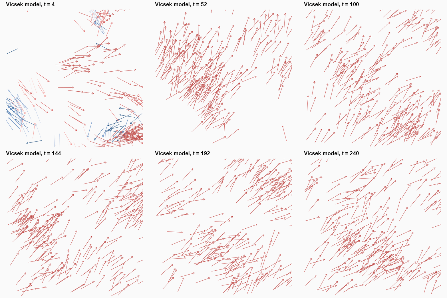
图 10 Vicsek 模型的实时演化(\(\eta=0.9\)):颜色是与瞬时全局平均方向的夹角余弦,所以「变红」就是群体对齐。 / Figure 10. The Vicsek model in real time (\(\eta=0.9\)): colour is the cosine between a heading and the instantaneous global mean, so “turning red” is the flock forming.
5.3 序参量随控制参数怎么变? / How does the order parameter move with the knob?
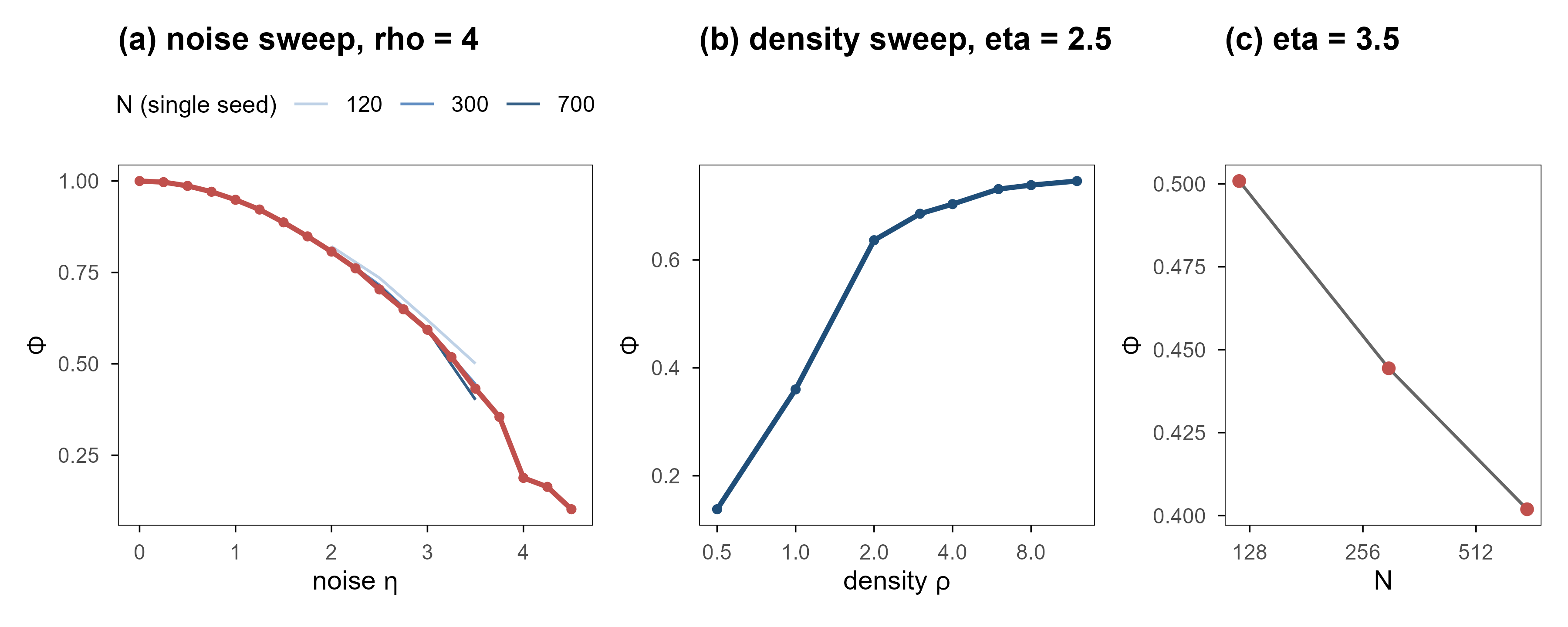
This is the central quantitative figure of the article. The left panel sweeps noise, the middle sweeps density, and the right isolates a hidden variable — system size. All three come from the same model and settings, with only the swept quantity changed.
Figure 6: 图 11 (a) 极化率随噪声下降;细线是不同系统尺寸的单次运行,\(N\) 越大曲线越低。(b) 固定 \(\eta=2.5\),提高密度同样可以把系统推入有序相。(c) 在 \(\eta=3.5\) 处把 (a) 的差异单独画出来:同一噪声下,系统越大越无序,说明小系统的「有序」是有限尺寸效应。 | Figure 11. (a) Polarisation falls with noise; thin lines are single runs at different system sizes, and larger \(N\) sits lower. (b) At fixed \(\eta=2.5\), raising the density also pushes the system into the ordered phase. (c) The same difference isolated at \(\eta=3.5\): at fixed noise, larger systems are less ordered, so the apparent order of small systems is a finite-size effect.
The thick line on the left is the mean over two seeds at \(N=300\); the three thin lines are single seeds at \(N=120, 300, 700\). Honesty is required here: at \(N=300\) there is no sharp transition — \(\Phi\) falls smoothly from 1.00 to 0.10. The thin lines give half of the reason: near \(\eta=3.5\) the \(N=120\) system still reports \(\Phi=\) 0.501, while \(N=700\) reports only 0.402. The higher order parameter of the small system is a finite-size effect, not stronger order.
The middle panel gives a cleaner conclusion: at \(\eta=2.5\), raising the density from \(\rho=0.5\) to \(\rho=12\) lifts \(\Phi\) from 0.138 to 0.746, with most of the change between \(\rho=0.5\) and \(4\). Order is not decided by one parameter but by the product of neighbour number and neighbour reliability. At low density each particle has few neighbours, so the local average is drowned by individual noise; raising density is equivalent to raising the signal-to-noise ratio of that average.
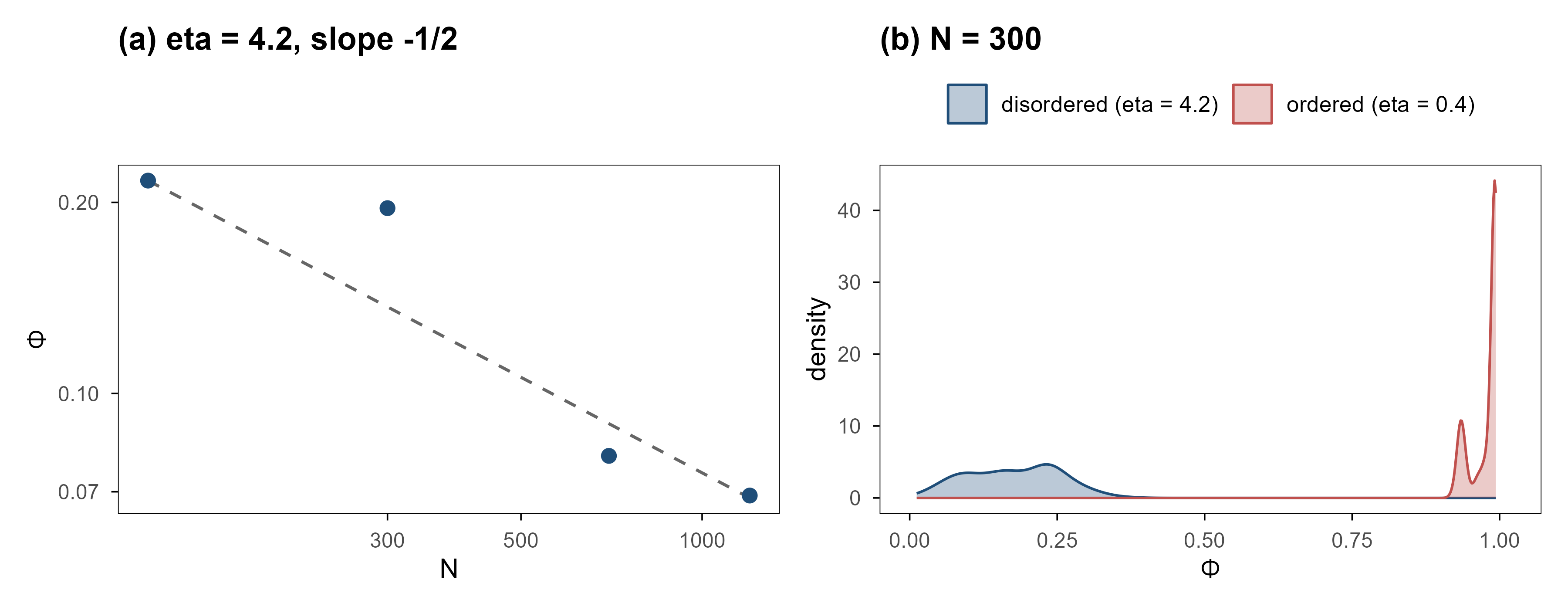
If the sweep stops at \(N=700\), “small systems look more ordered” is just a phenomenon. Push it to \(N=1200\) and look only at the disordered phase, and the statement becomes something a formula can be checked against.
Code
fsum <-subset(fl$summary, eta ==4.2)fsum$pred <- fsum$mean_phi[fsum$N ==120] *sqrt(120/ fsum$N)p_a <-ggplot(fsum, aes(N, mean_phi)) +geom_line(aes(N, pred), colour = em_pal[["grey"]], linetype ="dashed",linewidth =0.6) +geom_point(colour = em_pal[["deep_blue"]], size =2.4) +scale_x_log10() +scale_y_log10() +labs(x ="N", y =expression(Phi), title ="(a) eta = 4.2, slope -1/2")fhist <-subset(fl$series, N ==300& t >100)fhist$phase <-ifelse(fhist$eta <1, "ordered (eta = 0.4)","disordered (eta = 4.2)")fill_vals <-c("ordered (eta = 0.4)"= em_pal[["deep_red"]],"disordered (eta = 4.2)"= em_pal[["deep_blue"]])p_b <-ggplot(fhist, aes(phi, fill = phase, colour = phase)) +geom_density(alpha =0.3, linewidth =0.5) +scale_fill_manual(values = fill_vals, name =NULL) +scale_colour_manual(values = fill_vals, name =NULL) +coord_cartesian(xlim =c(0, 1.02)) +labs(x =expression(Phi), y ="density", title ="(b) N = 300")p_a + p_bfit_slope <-coef(lm(log(mean_phi) ~log(N), data = fsum))[[2]]
Figure 7: 图 12 无序相里的「有序」有多少是尺寸造的。左:\(\eta=4.2\) 的稳态极化率随 \(N\) 在双对数坐标下下降,虚线是由 \(N=120\) 出发、按 \(N^{-1/2}\) 外推的参考线;四个点整体沿着这条线走,中间两点在线的两侧。右:\(N=300\) 时 \(\Phi\) 的分布,有序相是一个贴着 1 的窄峰,无序相是一个横跨 0.01–0.37 的宽分布。 | Figure 12. How much of the ‘order’ in the disordered phase is manufactured by system size. Left: steady-state polarisation at \(\eta=4.2\) against \(N\) on log-log axes; the dashed line is the \(N^{-1/2}\) prediction anchored at \(N=120\), and the four points follow it overall, with the middle two falling on either side. Right: the distribution of \(\Phi\) at \(N=300\); the ordered phase is a narrow peak against 1, the disordered phase a broad distribution spanning 0.01–0.37.
The left panel gives a crisp number: at \(\eta=4.2\), \(\Phi\) drops from 0.216 at \(N=120\) to 0.069 at \(N=1200\); the ratio is 0.32 against \(1/\sqrt{10}=0.32\), and a log-log fit through the four points gives a slope of -0.56, close to \(-0.5\). The order parameter in the disordered phase is not zero; it shrinks as \(1/\sqrt{N}\) — which is exactly what “finite-size effect” means quantitatively: any finite system reports a little order, and the smaller the system, the bigger that little bit. One caveat is required: the middle two points do not sit on the line, so \(1/\sqrt{N}\) is a trend law here, not a pointwise one.
The right panel supplies the other half: at the same \(N=300\), \(\Phi\) in the ordered phase is a narrow peak against 1, while the disordered phase gives a broad distribution. One should not casually extend the claim to the fluctuations: the measured standard deviation only falls from 0.086 to 0.043, a ratio of 0.50, slower than \(1/\sqrt{10}\). The mean is predictable; the convergence rate of the fluctuations is not pursued here.
5.4 相图:把两条曲线合成一张地图 / The phase diagram: two curves into one map
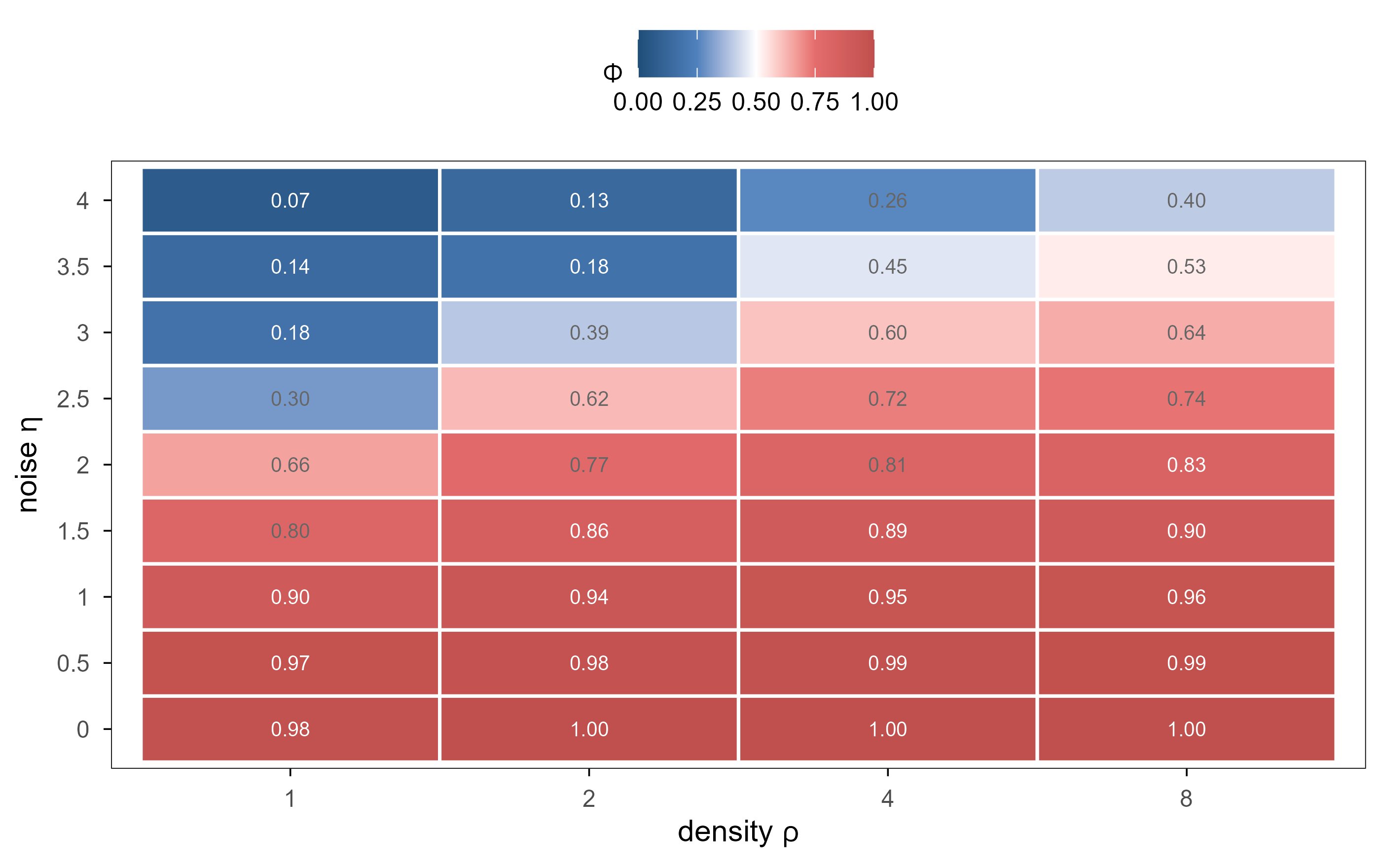
Figure 8: 图 13 Vicsek 模型的相图。颜色为稳态极化率 \(\Phi\),横轴为密度、纵轴为噪声。有序区(红)与无序区(蓝)之间是一条弯曲的边界:噪声越大,需要越多的邻居才能维持对齐。 | Figure 13. The Vicsek phase diagram. Colour is the steady-state polarisation \(\Phi\); the axes are density and noise. The boundary between the ordered region (red) and the disordered one (blue) is curved: the more noise, the more neighbours are needed to sustain alignment.
This figure folds the two sweeps into one two-dimensional map, read like a topographic map: the denser the contours, the more sensitive the system. For \(\eta\le 1\) almost every density is ordered; for \(\eta\ge 3.5\) only \(\rho\ge 4\) retains partial order; between them lies a diagonal band. Whether that band is a true transition depends on whether it narrows to a line as \(N\to\infty\) — the system sizes here cannot answer that, and the limitation has to be stated.
5.5 一级还是二级?一个没做完的检验 / First order or continuous? A test not completed here
A cautionary property of the Vicsek model in the literature is that at larger sizes the transition often appears first order, with hysteresis: increasing noise from the ordered side and decreasing it from the disordered side give different critical values, and in between the ordered and disordered phases coexist in bands.
This article does not run the hysteresis experiment, nor the reverse sweep starting from the ordered phase, so it cannot claim which type of transition is observed. The only defensible statement is: in this sweep at \(N=300\), \(\Phi(\eta)\) is a smooth, monotone decrease with no sign of a jump or of bistability. That may be because the system is too small (a first-order transition is heavily smeared by finite size) or because the parameter grid is too coarse. The point of saying it is to stop the reader from reading the gradient in Figure 13 as a critical point.
5.6 三维:规则里根本没有「二维」 / Three dimensions: the rule never mentioned “two”
Code
library(plotly)mk3d <-function(k) { d <- vic3$runs[[k]]plot_ly(d, x =~x, y =~y, z =~z, color =~alignment,colors =colorRamp(em_div), type ="scatter3d", mode ="markers",marker =list(size =2.2), hoverinfo ="text",text =~sprintf("alignment %.2f", alignment)) |>layout(title =sprintf("%s (Phi = %.2f)", k, vic3$phi[[k]]),showlegend =FALSE,scene =list(xaxis =list(title ="", showticklabels =FALSE),yaxis =list(title ="", showticklabels =FALSE),zaxis =list(title ="", showticklabels =FALSE),aspectmode ="cube"),margin =list(l =0, r =0, t =30, b =0))}subplot(mk3d("eta 0.2"), mk3d("eta 0.8"), mk3d("eta 1.6"),nrows =1, shareX =FALSE, shareY =FALSE, titleX =FALSE, titleY =FALSE)
Figure 9: 图 14 三维 Vicsek(可拖动旋转)。三种噪声下同一密度、同一速度的末态;每个点是一个粒子的位置,颜色为与全局平均方向的夹角余弦。三维版本的意义不是「更好看」,而是说明规则中没有任何与维度有关的内容。 | Figure 14. Three-dimensional Vicsek (drag to rotate). Final states at one density and speed under three noise levels; each dot is a particle, coloured by the cosine between its heading and the global mean. The point of the 3-D run is not that it looks better, but that nothing in the rule refers to the dimension.
The 3-D results agree with the 2-D ones: \(\Phi=\) 0.998 at noise \(0.2\), 0.973 at \(0.8\), 0.894 at \(1.6\). The numbers themselves matter little; what matters is that the same rule works in three dimensions, showing that alignment is a mechanism independent of spatial dimension. Living systems are not confined to two dimensions, and models often forget it.
6. 简单细胞通讯如何产生空间图案? / How Can Simple Cell Communication Produce Spatial Patterns?
The macroscopic structures in the previous two sections were alignment or connected patches. A more common biological structure is spatial pattern: zebra stripes, hair follicle spacing, the gaps between fingers, veins on a fly wing. Turing (1952) gave a counter-intuitive mechanism: two chemicals, one activating itself and one inhibiting it while diffusing faster, suffice to grow a pattern with a characteristic wavelength out of a uniform state.
6.1 模型:局部激活 + 长程抑制 / The model: local activation, long-range inhibition
Treat each site as a cell with a substrate \(u\) and a signal \(v\). The cell converts \(u\) into \(v\), and \(v\) catalyses that conversion (positive local feedback), while \(v\) diffuses to the neighbours and suppresses the same reaction there (negative long-range feedback). The Gray–Scott equations are the most compact statement of this idea:
The two diffusion constants satisfy \(D_u>D_v\) (substrate fast, signal slow), which is the lattice version of the Turing condition: inhibition must travel further than activation. \(F\) is the feed rate, \(k\) the kill rate, and together they decide which morphology the system settles into.
6.2 为什么「扩散」会制造结构? / Why would diffusion create structure?
Intuitively diffusion erases differences: ink dropped into water spreads out, it does not gather into spots. Turing’s counter-intuitive point is that when two species diffuse at different rates and regulate each other, diffusion can destroy the uniform state instead.
Linearise the equations around the uniform steady state \((u^*,v^*)\) and insert a perturbation \(e^{\sigma t+i\mathbf{k}\cdot\mathbf{x}}\); the dispersion relation is
where \(J\) is the Jacobian of the reaction terms and \(\kappa=|\mathbf{k}|\) the wavenumber. Note that \(\kappa^2\) appears only inside the diffusion terms: if \(D_u=D_v\), diffusion shifts \(\sigma\) uniformly and can never turn stability into instability. Only when \(D_u\neq D_v\) and the signs of \(J\) encode “self-activation plus cross-inhibition” does \(\sigma\) become positive at some finite wavenumber \(\kappa_c\) — this is diffusion-driven instability.
The derivation makes two testable predictions, and both are visible in the experiments here. First, a preferred wavenumber exists, so the spot spacing is nearly uniform (Figure 15). Second, patterns exist only in a narrow band of parameters, because outside it either \(J\) itself is unstable (the whole lattice ignites) or diffusion is too weak to break stability (nothing grows). This also explains why Figure 18 has 16 combinations with a pattern and 60 without one.
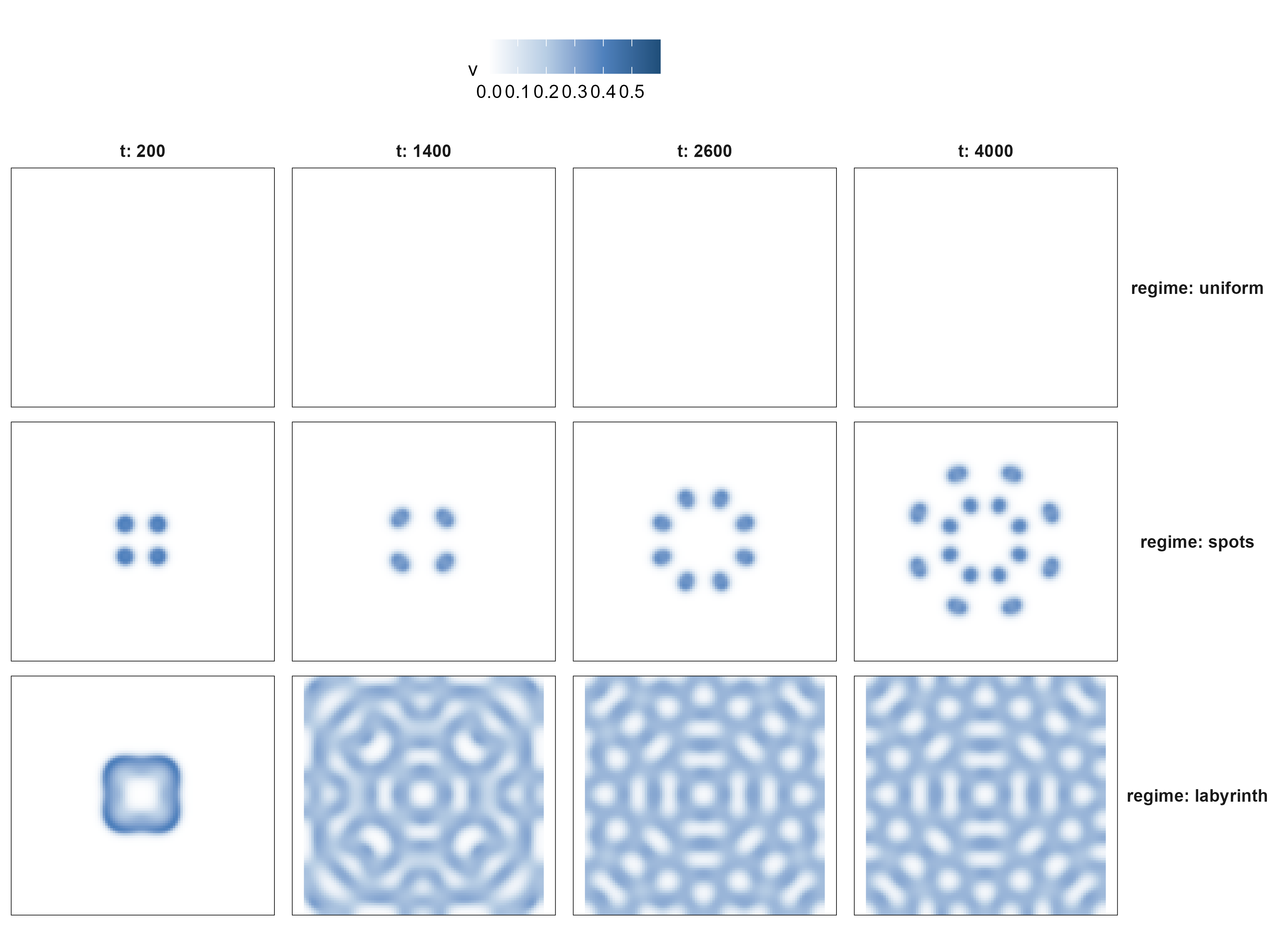
Figure 10: 图 15 同一模型、同一初始种子,只改 \((F,k)\)。上行:信号始终无法自我维持,系统回到均匀态;中行:斑点;下行:迷宫状的条纹。每列是同一时刻。颜色为信号浓度 \(v\)。 | Figure 15. The same model and the same initial seed, changing only \((F,k)\). Top: the signal cannot sustain itself and the lattice returns to uniform. Middle: spots. Bottom: labyrinthine stripes. Columns are matched in time; colour is the signal \(v\).
Code
do.call(rbind, lapply(names(pat), function(nm) { m <- pat[[nm]]$metricsdata.frame(regime = nm, F = pat[[nm]]$F, k = pat[[nm]]$k,`signal fraction`=round(m$v_frac[nrow(m)], 3),patches =as.integer(m$patches[nrow(m)]),`autocorr. lag`=as.integer(m$ac_len[nrow(m)]),class =pattern_class(pat[[nm]]$final))})) |> knitr::kable()
Table 3: 三种组织在 \(t=4000\) 时的宏观量。autocorr. lag 是水平自相关首次降到 \(1/e\) 的格点数。
regime
F
k
signal.fraction
patches
autocorr..lag
class
uniform
0.010
0.060
0.000
0
28
uniform
spots
0.035
0.065
0.068
16
5
spots
stripes
0.030
0.055
0.620
1
4
labyrinth
English: macroscopic variables of the three tissues at \(t=4000\).
The only difference between the three rows is two numbers: \(F\) and \(k\). No row was “programmed” to be spots or a labyrinth — spots grew at \(F=0.035\), \(k=0.065\), and the labyrinth at \(F=0.030\), \(k=0.055\). This is worth pausing on: the type of pattern is not set by any higher-level instruction, but by the ratio of two reaction rates.
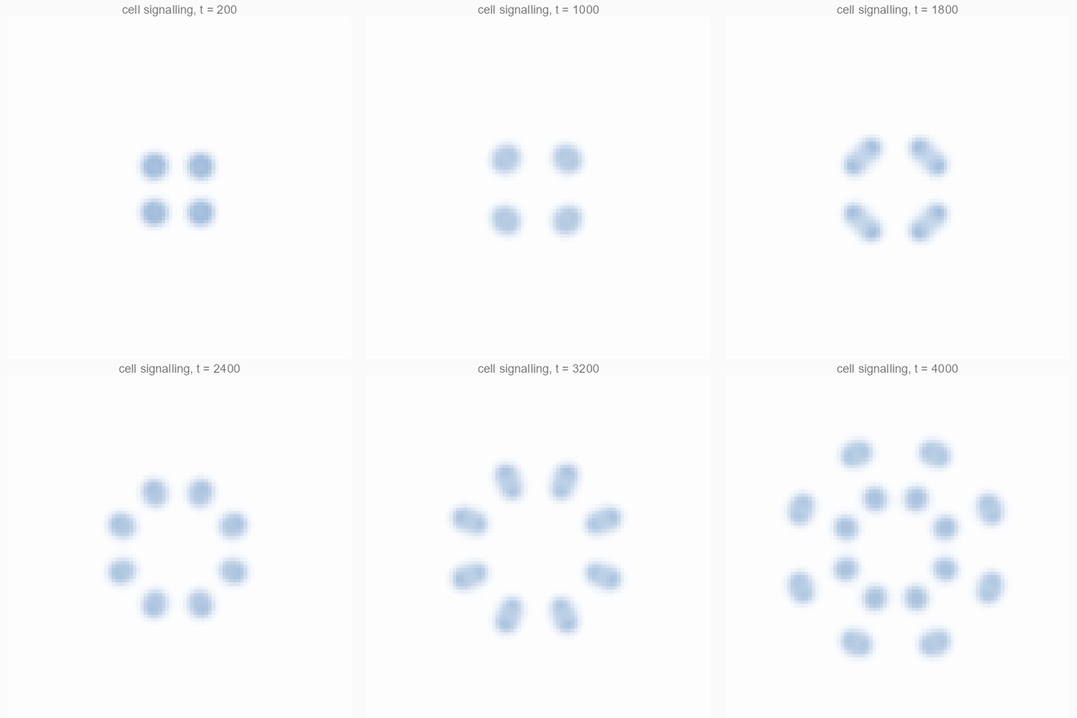
图 16 斑点图案的生长过程(\(F=0.035\),\(k=0.065\))。从一个方形种子的局部扰动开始,信号向外扩散、彼此抑制,最后稳定成一群体积相近的斑点。 / Figure 16. How spots grow (\(F=0.035\), \(k=0.065\)). Starting from one square perturbation, the signal spreads, inhibits its neighbours, and settles into a set of spots of similar size.
The easily missed point in Figure 16 is that the spots are nearly the same size. That is the signature of the Turing mechanism: the wavelength is set by the ratio \(\sqrt{D_u/D_v}\) of the diffusion constants, not by the shape or size of the initial seed. In other words, the scale is encoded in the parameters, not in the initial condition.
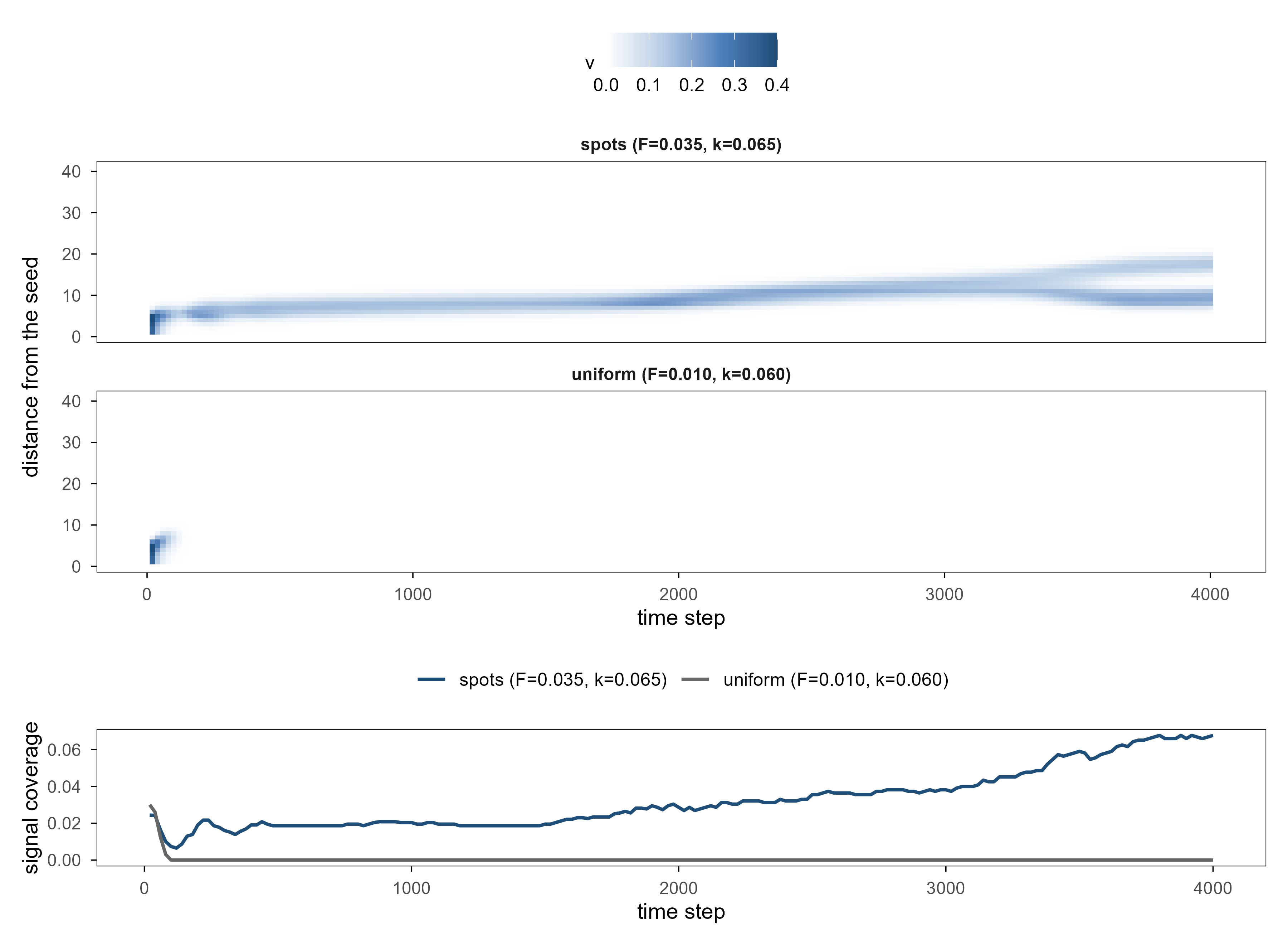
An animation shows only what the lattice ends up looking like. To see how it grows, a space-time diagram (kymograph) is better: take one row of the lattice and stack its concentration profile at successive times.
Figure 11: 图 17 同一方程的时空图:横轴是时间(0–4000 步),纵轴是距种子中心的距离,颜色是该半径上的平均信号浓度(按环平均,把角度方向压掉)。上:\((F,k)=(0.035,0.065)\),信号从中心向外推进,前沿过处留下等间距的波列,间距由参数决定、与初始种子无关;下:\((F,k)=(0.010,0.060)\),同一初始扰动在几百步内衰减为零。最下一行是两者的信号覆盖率随时间的变化。 | Figure 17. Space-time diagrams of the same equation: time runs left to right (0–4000 steps), the vertical axis is distance from the centre of the seed, and colour is the signal averaged over rings at that radius (which removes the angular direction). Top: \((F,k)=(0.035,0.065)\), where the signal advances outwards and leaves an evenly spaced wave train behind its front, the spacing set by the parameters rather than the seed. Bottom: \((F,k)=(0.010,0.060)\), where the same initial perturbation decays to zero within a few hundred steps. The lowest panel tracks signal coverage over time for both.
The space-time diagram settles two things at once. First, the pattern is grown, not placed: the signal advances outwards, and the radial profile at \(t=4000\) has one peak at about 7 lattice sites and another at about 17, roughly 10 sites apart — the Turing wavelength, fixed by the parameters and independent of the seed’s shape or size. Second, growth has a time scale: coverage rises monotonically from 2.0% at \(t=1000\) to 6.8% at \(t=4000\), and the patch count grows from 4 to 16, while the control case decays to zero within 80 steps.
6.4 相图:图案在哪里出现? / The phase diagram: where do patterns exist?
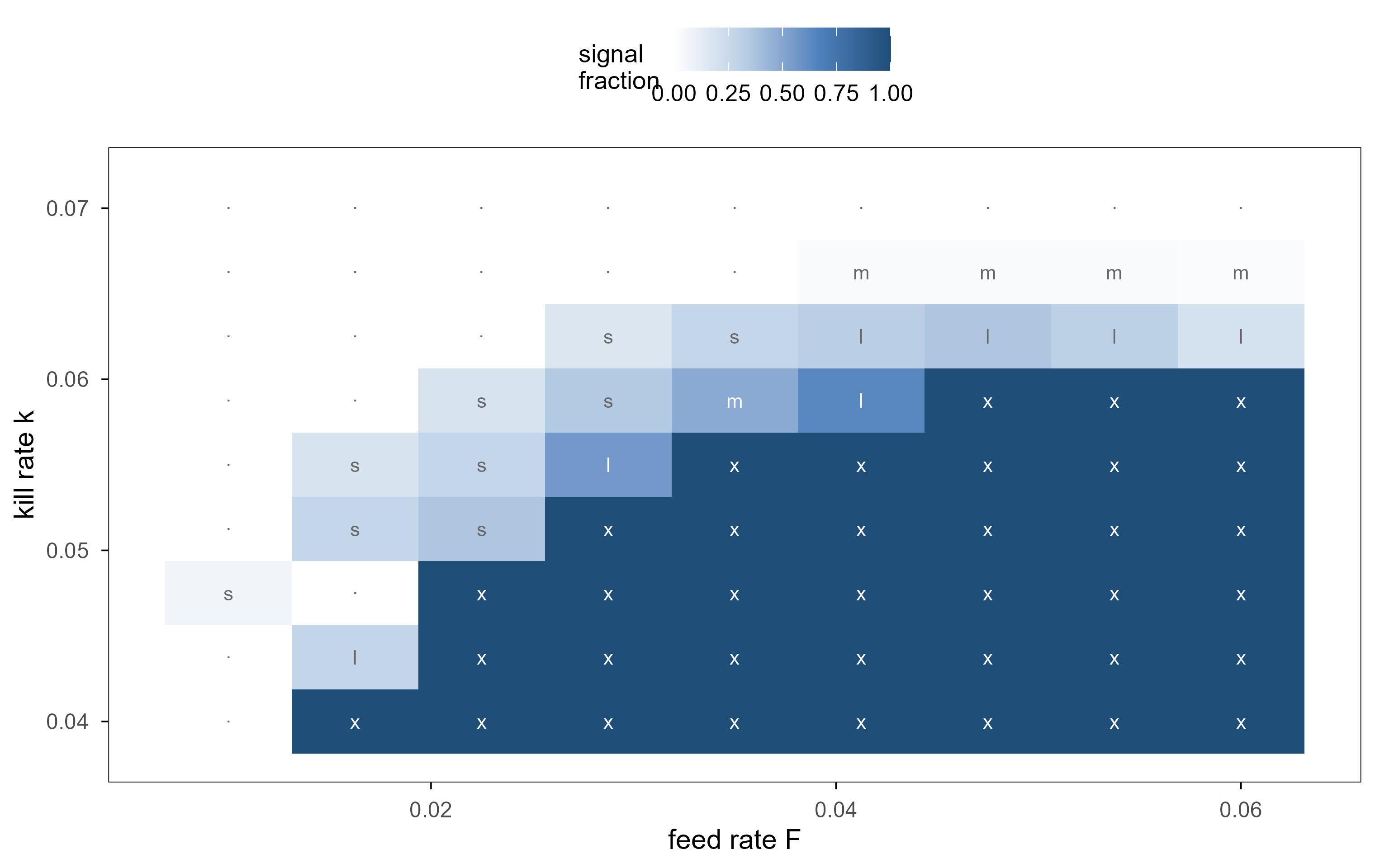
Figure 12: 图 18 细胞通讯模型的参数地图。颜色为稳态时携带信号的格点比例;标注为该格点的形态:· 均匀(什么都不长),s 斑点,l 迷宫(单连通条纹),m 混合,x 整片饱和。左下角(低补给)信号无法维持;右上角(高补给、低清除)整片格点被点亮;中间的窄带才是斑点与条纹。 | Figure 18. Parameter map of the signalling model. Colour is the fraction of the lattice carrying signal at steady state; the label gives the morphology: · uniform (nothing grows), s spots, l stripes, m mixed, x saturated. The lower-left corner (low feed) cannot sustain a signal; the upper-right (high feed, low kill) ignites the whole lattice; only the narrow band between them contains spots and stripes.
The figure shows that “pattern” is a narrow-band phenomenon: in the \(9\times 9\) scan, 9 parameter combinations give spots, 7 give a labyrinth, 24 give nothing, and 36 light up the whole lattice. In most of parameter space nothing happens — the opposite of the impression that complex systems always produce complex behaviour.
One more caveat: the “labyrinth” and the spots here are two solutions of the same equation, not two mechanisms. That is a warning: inferring “different mechanism” from “different morphology” is unsafe. Inside a model we can verify common ancestry; in a real tissue we cannot.
Seen from another angle the same map is easier to read: plot the coverage as height and parameter space becomes a plateau (fully saturated) plus a plain (nothing grows), separated by a steep slope running along the diagonal; spots and labyrinths appear only in a narrow strip on the face of that slope.
Figure 13: 图 19 图 18 的三维版本(可拖动旋转)。高度与颜色都是信号覆盖率,底面投影是对应的等高线。高原是「整片饱和」,平原是「什么都不长」,中间的陡坡上有图案——坡的宽度只有一两个参数格点。 | Figure 19. Figure 18 in three dimensions (drag to rotate). Height and colour are signal coverage; the projection on the floor is the corresponding contour map. The plateau is ‘fully saturated’, the plain is ‘nothing grows’, and the patterns live on the steep slope between them, whose width is only one or two parameter cells.
7. 如何判断一个系统真的发生了「涌现」? / How Do We Know a System Truly Exhibits Emergence?
By now there are three models and a dozen figures. The uncomfortable question can no longer be postponed: what entitles us to call these pictures emergence rather than decoration?
7.1 五项检查 / Five checks
本文使用五项检查,每一项都对应一个可计算的量,而不是一句形容词:
This article uses five checks, each tied to a computable quantity rather than an adjective:
序参量:存在一个只在集体尺度上定义的量,并且它随控制参数系统性地变化。 Order parameter: a quantity defined only collectively, which moves systematically with a control parameter.
空间尺度:结构的关联长度显著大于个体间距(否则只是「每个细胞各自兴奋」)。 Spatial scale: the correlation length is much larger than the spacing between units (otherwise it is just “each cell excited on its own”).
稳定性:结构在若干步之后仍然存在,而不是一闪而过。 Stability: the structure survives many updates instead of flashing once.
可复现性:换随机种子、换初始条件,同类结构仍然出现。 Reproducibility: the same kind of structure appears under a different seed or initial condition.
不可还原性:无法从任何单个个体的状态读出这个量。 Irreducibility: the quantity cannot be read off any single unit.
7.2 反例:熵最高、结构最少 / The counter-example: maximum entropy, minimum structure
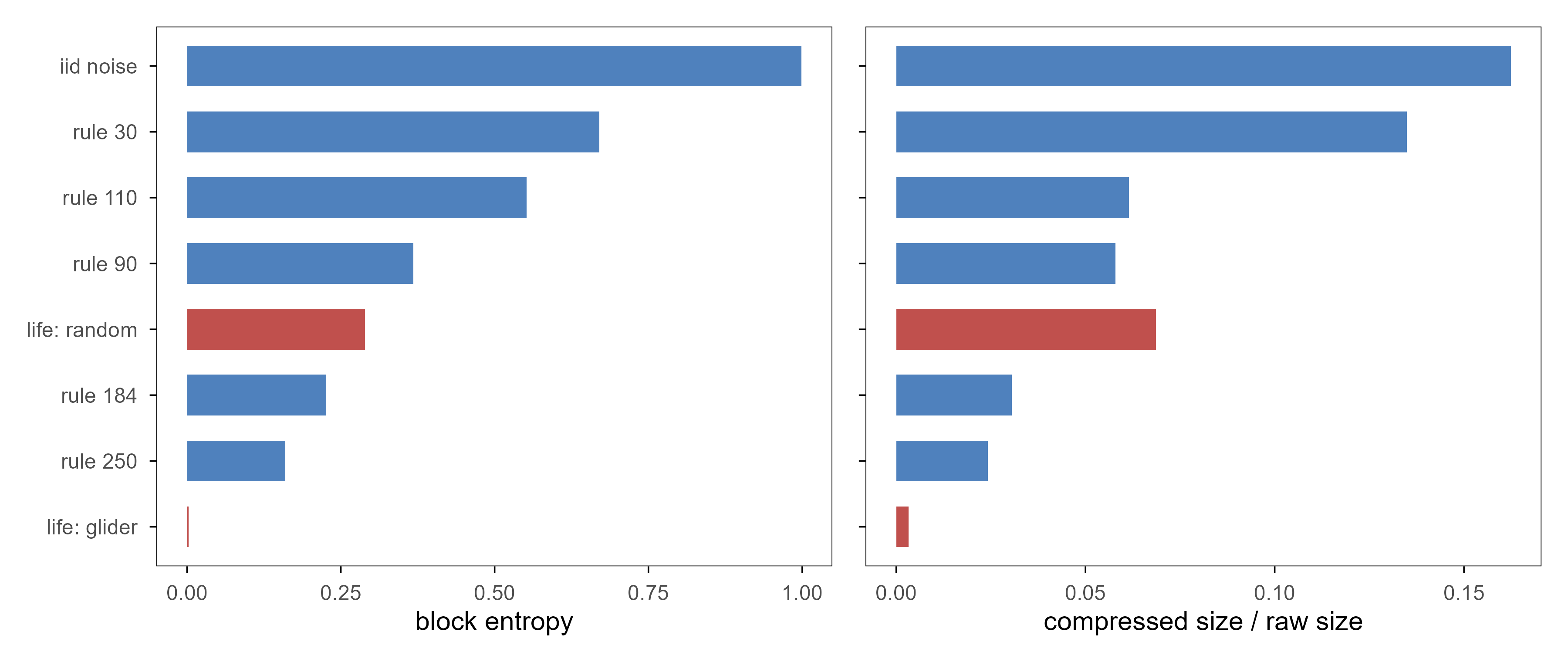
Figure 14: 图 20 八个系统的两个宏观量。左:块熵(局部构型有多不可预测);右:可压缩性(gzip 压缩后的体积比,越低越有规律)。iid 噪声的熵接近 1,但完全没有结构;rule 30 的熵也很高,而且逐帧毫无记忆;滑翔机的熵几乎为 0,却是一个稳定、可移动的宏观物体。熵高不等于涌现,熵低也不等于涌现。 | Figure 20. Two macroscopic quantities for eight systems. Left: block entropy (how unpredictable the local configuration is). Right: compressibility (compressed size over raw size; lower means more regular). iid noise has entropy near 1 but no structure at all; rule 30 also has high entropy and no frame-to-frame memory; the glider has almost zero entropy yet is a stable, mobile macroscopic object. High entropy is not emergence, and low entropy is not emergence either.
Figure 20 is the counter-example of the article. Sorted by block entropy, iid noise comes first (1.00), far above rule 30 (0.67) and the Game of Life (0.003). If “complex” meant entropy, random numbers would be the most complex system in the world — clearly not what we mean.
Compressibility takes another angle: iid noise barely compresses (0.162), rule 30 is slightly better (0.135), rule 110 is clearly more regular (0.062), and the glider is almost pure repetition (0.003). Compressibility measures description length; entropy measures uncertainty. They are not the same thing: a system can be hard to predict and easy to describe, or the other way round.
So no single criterion suffices. The conclusion of this article is: only when “the order parameter moves systematically with a parameter”, “the correlation length far exceeds the spacing”, and “the structure reproduces across seeds” all hold is it worth saying that “this system is emergent at this scale”. Miss one, and all you have is “a pattern appeared”.
Eight systems are still a hand-picked sample. Apply the same two metrics to all 256 elementary rules and you can see how they are distributed over rule space — and why “complex” cannot be collapsed into one number.
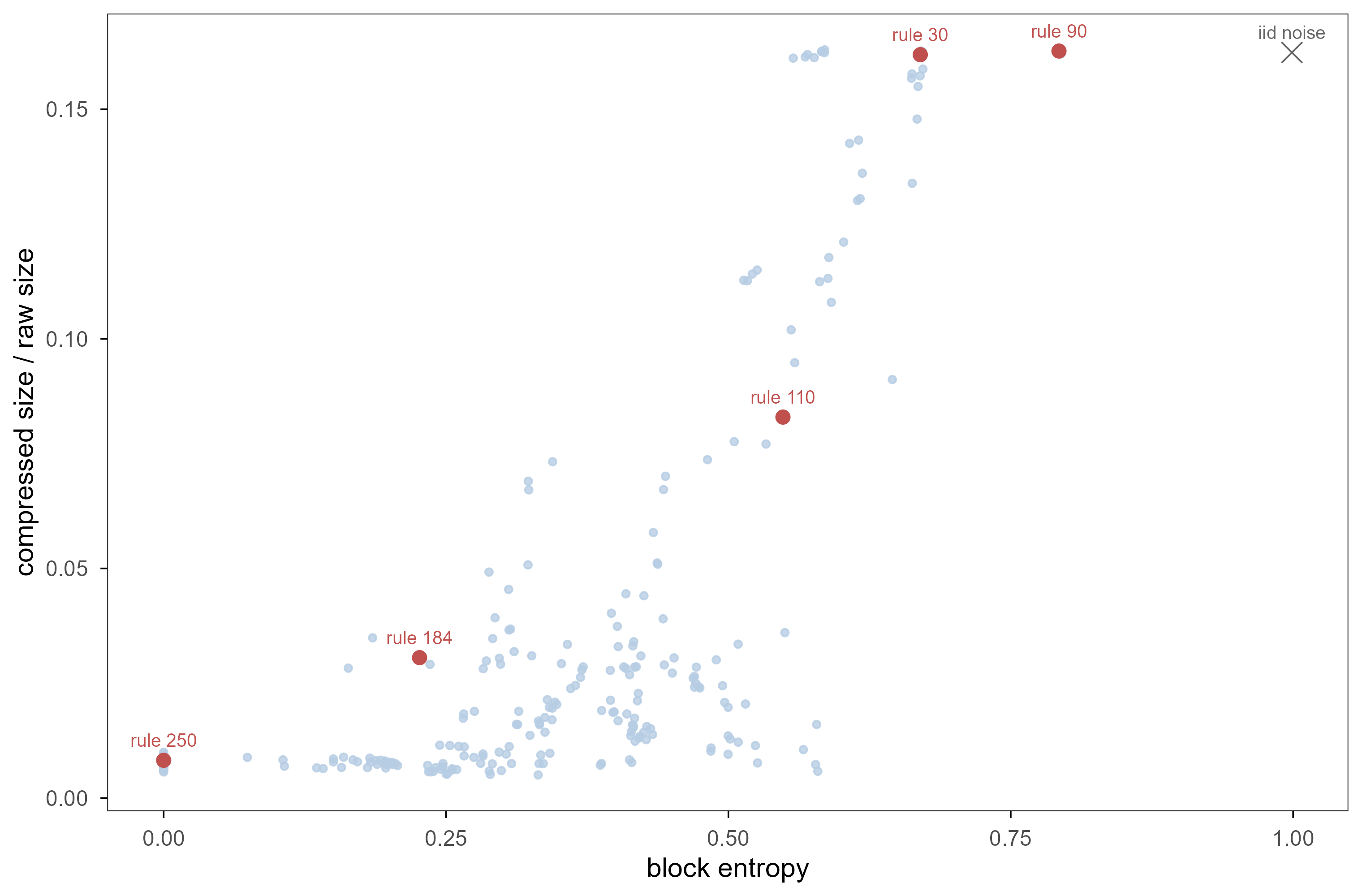
Figure 15: 图 21 把全部 256 条规则放进(块熵,可压缩性)平面,每条规则从同一随机初始行出发。浅蓝点是其余规则,红点是文中反复提到的五条,灰色叉号是一维 iid 噪声(同尺寸,可直接比较)。两个量正相关,但显然不是同一个轴:熵最高的规则是 rule 90(分形),而不是 rule 30;rule 110 与 rule 30 的熵接近,可压缩性却差一倍。 | Figure 21. All 256 rules placed in the (block entropy, compressibility) plane, each run from the same random initial row. Pale blue dots are the other rules, red dots the five discussed in the text, the grey cross is one-dimensional iid noise (same lattice size, so directly comparable). The two quantities are positively correlated, but they are clearly not the same axis: the highest-entropy rule is rule 90 (a fractal), not rule 30; rules 110 and 30 have similar entropy but their compressibility differs by a factor of two.
This scatter fills the half that Figure 20 leaves out. Figure 20 only shows that high entropy is not complexity; Figure 21 shows that in this metric system “complex” is at least two directions: the horizontal axis (entropy) measures local unpredictability, the vertical (compressibility) measures description length, and the two are correlated but not interchangeable. Rule 90 has the highest block entropy of all 256 rules (0.794), higher even than rule 30’s 0.670, yet its pattern is a fractal that can be written as a formula. Rules 30 and 110 have entropies of 0.670 and 0.548 but compressibilities of 0.162 and 0.083 — nearly a factor of two apart. “Hard to predict” and “hard to describe” are two different things, and emergence is a third.
8. 涌现、进化、非线性与信息 / Emergence, Evolution, Nonlinearity, and Information
8.1 非线性是必要条件,但不是充分条件 / Nonlinearity is necessary but not sufficient
In all three models \(F\) is nonlinear: a threshold in the Game of Life, a circular mean in Vicsek, a \(uv^2\) term in Gray–Scott. This is no accident. If \(F\) were linear, superposition would hold, every macroscopic quantity would be a weighted sum of microscopic ones, and any “new” macroscopic behaviour could be read directly off individual behaviour — by the definition in Section 2, that is not emergence.
But nonlinearity does not guarantee emergence. Rule 30 is strongly nonlinear and yet has almost no reproducible macroscopic structure (the counter-example of Section 7). Nonlinearity provides the possibility; the location in parameter space provides the realisation.
8.2 进化:选择作用在涌现出来的表型上 / Evolution: selection acts on emergent phenotypes
One easily missed fact about evolution: selection never acts on genes directly, it acts on phenotypes — and phenotypes are almost entirely emergent quantities: organ shape, tissue mechanics, collective behaviour. At the gene level there is only a sequence of bases; there is no “wing”.
这就产生了一个回路:涌现出来的宏观结构一旦稳定,就变成新的选择单位(units of selection),反过来约束微观规则。生命游戏里的滑翔机可以相互碰撞、被破坏,这就是一个(极其简化的)选择场景:能在碰撞中保持自身结构的滑翔机「活下来」。真实的进化比这复杂得多,但机制的形状是一样的。
This closes a loop: once an emergent macroscopic structure is stable, it becomes a new unit of selection and constrains the microscopic rules in turn. Gliders in the Game of Life can collide and be destroyed — a (very simplified) selection scenario in which gliders that keep their structure through collisions “survive”. Real evolution is far more complex, but the shape of the mechanism is the same.
8.3 信息:三种不同的量 / Information: three different quantities
「信息」在这类讨论里经常被混用,至少有三件事需要分开:
“Information” is used loosely in these discussions, and at least three things must be separated:
熵(entropy):局部构型的不确定性。iid 噪声最高,滑翔机最低。 Entropy: uncertainty of the local configuration. Highest for iid noise, lowest for a glider.
描述长度(description length):压缩这个系统需要多少比特。它与熵相关但不等价(第 7 节)。 Description length: how many bits are needed to compress the system. Related to entropy but not identical (Section 7).
因果涌现(causal emergence):宏观变量对未来的预测能力是否强于微观变量。Hoel 等人(2013)给出了一个可操作的度量:比较宏观与微观两种描述下的有效信息量。 Causal emergence: whether a macroscopic variable predicts the future better* than the microscopic one. Hoel et al. (2013) give an operational measure comparing effective information at the two scales.*
The third is closest to the question of this article and the easiest to overstate. It does have a rigorous definition, but it requires specifying how the macroscopic variable is coarse-grained, and that choice is itself a modelling decision — change the coarse-graining and the conclusion can flip. This matches Section 3: macroscopic variables are chosen by us, not handed down by nature.
8.4 为什么生命系统几乎天然带有涌现 / Why living systems are almost inevitably emergent
A basic feature of life is multi-scale organisation: molecule → organelle → cell → tissue → organ → organism → group. Every level has its own variables, its own time scale, its own invariants. A level cannot be restated in the language of the level below, not because of anything mystical, but because the set of variables has changed.
The Vicsek result in Section 5 gives a concrete version: “how many neighbours” and “how reliable a neighbour is” are interchangeable. At the cell level this corresponds to density and signalling noise; at the tissue level to cell number and junction strength. The same mathematical relation recurs at different scales, which is both why simple models of life work and why they are dangerous — the model can be right while the scale is wrong.
9. 对 AI 与「活模型」的启发 / Implications for AI and “Living Models”
9.1 涌现这个词在 AI 里被用得太松 / The word is used too loosely in AI
2022 年以来,「涌现能力(emergent abilities)」成了大模型文献里的高频词:某些能力在小模型上为零,过了某个规模突然出现(Wei et al., 2022)。但这个结论对度量方式极其敏感。Schaeffer 等人(2023)指出,很多所谓的「突然出现」来自非线性或不连续的评分指标:把精确匹配换成 token 级准确率,曲线就变成平滑上升。
Since 2022, “emergent abilities” has become a fixture of the large-model literature: some capability is zero in small models and appears abruptly past a certain scale (Wei et al., 2022). But that conclusion is extremely sensitive to the metric. Schaeffer et al. (2023) show that many such “jumps” come from nonlinear or discontinuous scoring: replace exact match by token-level accuracy and the curve becomes a smooth rise.
This is exactly the lesson of Section 7: without a pre-declared macroscopic quantity there is no testable claim of emergence. “The model suddenly can do X” and “our score is steep in some range” can look identical in the data.
9.2 多智能体:局部规则的设计问题 / Multi-agent systems: designing the local rule
The lesson of the Vicsek model for multi-agent systems is concrete rather than rhetorical. Suppose you have a population of agents, each seeing only a few peers, and you want the whole to converge on one conclusion. Section 5 gives three things:
对齐强度与噪声必须匹配:交互半径太小或噪声太大,局部平均不可靠,系统停在无序相。 Alignment strength must match noise: too small a radius or too much noise makes the local average unreliable and the system stays disordered.
密度是可以调的控制参数:增加可见同伴的数量,等价于降低噪声。 Density is a control parameter: increasing the number of visible peers is equivalent to reducing noise.
有限尺寸会骗人:小群体看起来更一致,这只是因为 \(1/\sqrt{N}\) 的涨落更大。 Finite size deceives: small groups look more consistent only because \(1/\sqrt{N}\) fluctuations are larger.
The third is especially dangerous in engineering: a 20-agent system that “shows consensus” does not imply that a 2000-agent system will. The direction is the opposite — in the finite-size experiment here, larger systems are less ordered at the same noise.
9.3 「活模型」需要的是规则,不是蓝图 / “Living models” need rules, not blueprints
To compress Sections 4–6 into one design principle: do not specify the macroscopic behaviour directly; design the local interaction rule, and treat the macroscopic quantities as outputs to be measured.
This is the opposite of mainstream end-to-end supervision. An end-to-end model treats macroscopic behaviour as a training target (say, “predict the next frame of the crowd”) and therefore learns macroscopic correlations without the mechanism that generates them; under distribution shift the correlations fail. A rule-based model (cellular automaton, Vicsek, reaction–diffusion) instead generates new macroscopic behaviour when parameters change, including behaviour never seen in training.
9.4 边界:什么不能从这些模型里学到 / The boundary: what these models cannot teach
Three things these models cannot teach must be stated. First, they have no objective: they optimise nothing, whereas organisms and agents optimise (fitness, reward, free energy). Second, they do not learn: the rules are fixed, whereas real collective behaviour changes with experience. Third, they have no semantics: a glider “means” nothing, whereas signals between cells have biological meaning.
So the right statement is not “life is a cellular automaton” but: cellular automata and the Vicsek model give a lower bound on the necessary conditions for the step from rules to structure. Life also needs objectives, learning and semantics — three other articles.
9.5 没有中央控制器,谁来保证「一致到正确」? / Without a controller, who guarantees that consensus is correct?
The success of the Vicsek model is easily misread as “decentralised is always better”. Only one thing is guaranteed: the particles converge on a common heading. Nothing guarantees that this heading is the one we want — rotate every initial heading by \(180^\circ\) and the system converges just as happily, to the opposite direction. Alignment is a mechanism for consensus, not for correctness.
This is fatal for multi-agent systems. If every agent pulls its judgement towards the mean of its neighbours, a sufficiently large initial bias is amplified into consensus rather than corrected, as long as the noise does not erase it. The more aligned the system, the weaker its error correction, because a deviating individual carries less and less weight in the local average. Nothing in the model here checks facts, so it cannot distinguish “everyone agrees” from “everyone is right”.
Making collective behaviour both emergent and reliable needs at least two things: heterogeneity (not every unit follows the same rule) and contact with the world (at least some units update from verifiable signals rather than from neighbours alone). Neither is in the models here, and they are precisely the difference between biological groups and engineered ones: a flock hits obstacles, a cell dies, whereas a population of purely imitating agents pays no price at all.
10. 结论:复杂性不是被写进去的,而是被组织出来的 / Conclusion: Complexity Is Not Merely Written In, but Organized Out
Code
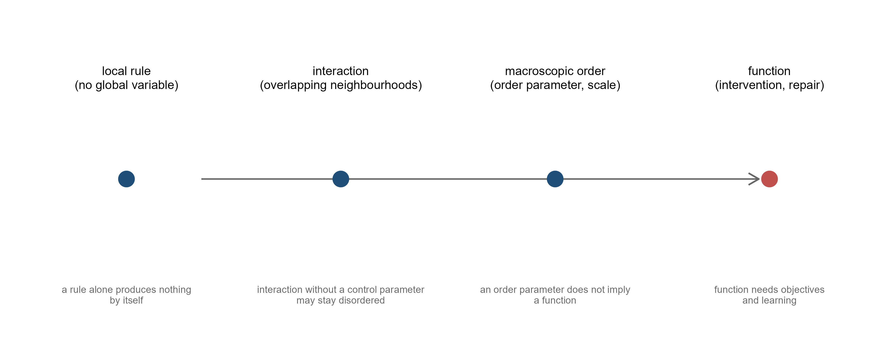
ladder <-data.frame(x =1:4,label =c("local rule\n(no global variable)","interaction\n(overlapping neighbourhoods)","macroscopic order\n(order parameter, scale)","function\n(intervention, repair)"),caveat =c("a rule alone produces nothing\nby itself","interaction without a control parameter\nmay stay disordered","an order parameter does not imply\na function","function needs objectives\nand learning"))ggplot(ladder) +geom_segment(aes(x =1.35, xend =3.95, y =0.5, yend =0.5),arrow =arrow(length =unit(3, "mm")), colour = em_pal[["grey"]],linewidth =0.5) +geom_point(aes(x, y =0.5, colour = x <=3), size =5) +geom_text(aes(x, y =0.78, label = label), size =3.1, lineheight =0.95) +geom_text(aes(x, y =0.18, label = caveat), size =2.5, colour = em_pal[["grey"]],lineheight =0.9) +scale_colour_manual(values =c(`FALSE`= em_pal[["deep_red"]],`TRUE`= em_pal[["deep_blue"]]),guide ="none") +coord_cartesian(xlim =c(0.6, 4.4), ylim =c(0.05, 0.95)) +theme_void()
Figure 16: 图 22 全文的一张总图。从左到右四层:局部规则、交互结构、宏观量(这三层由本文的实验覆盖,蓝点),以及功能与干预(需要目标与学习,超出本文范围,红点)。每个点下方写的是这一层不能保证的东西。 | Figure 22. The whole article in one picture. Four layers from left to right: local rule, interaction structure, macroscopic quantities (the three covered by the experiments here, blue dots), and function / intervention (which needs objectives and learning and lies outside this article, red dot). Under each dot is what that layer does not guarantee.
把全文压缩成四句话:
The whole article in four sentences:
局部规则决定「可能发生什么」。规则里没有的宏观行为,不会自己出现。 The local rule decides what can happen. A macroscopic behaviour absent from the rule will not appear by itself.
交互结构决定「信息能传多远」。邻域重叠是长程关联的唯一来源。 The interaction structure decides how far information travels. Overlapping neighbourhoods are the only source of long-range correlation.
尺度提升决定「什么算一个量」。序参量、关联长度、连通块都是在这个步骤被定义的。 The change of scale decides what counts as a quantity. Order parameters, correlation lengths and components are defined at this step.
测量决定「我们有没有资格说它存在」。没有事先声明的宏观量,就没有可检验的涌现主张。 Measurement decides whether we are entitled to say it exists. Without a pre-declared macroscopic quantity there is no testable claim of emergence.
If a reader wants to claim emergence in their own system, the workflow here compresses into five items. Each maps to a concrete practice in this article rather than to an abstract principle:
写下规则:\(F\)、邻域、更新顺序,以及边界条件。 Write the rule down: \(F\), the neighbourhood, the update order, the boundary conditions.
写下宏观量的公式,并说明它为什么是对称的、为什么不能从个体读出。 Write the formula for the macroscopic quantity, and say why it is symmetric and why it cannot be read off individuals.
扫描参数并报告范围,包括「什么都不发生」的那一端——负对照。 Sweep the parameter and report the range, including the end where nothing happens: the negative control.
报告系统尺寸与种子数,并把有限尺寸效应单独画出来,最好按 \(1/\sqrt{N}\) 检验一次。 Report system size and the number of seeds, plot the finite-size effect separately, and if possible test it against \(1/\sqrt{N}\).
给出一个反例:一个看起来同样复杂、但宏观量不支持涌现的系统。 Give a counter-example: a system that looks equally complex but whose macroscopic quantities do not support emergence.
None of the five needs sophisticated technique, but together they block most “it looks complex, therefore it is emergent” conclusions. Section 7 of this article is organised exactly this way: the five checks (7.1), the counter-example (7.2), and the comparison figures that put them side by side (Figures 20 and 21).
Back to the opening question: is the complexity we see determined by the rules themselves, or shaped jointly by interaction, scale and organisation? The experiments here answer “the latter”, with one important qualification: the rule sets the boundary of what is possible. No parameter choice makes the Vicsek model produce stripes, and none makes Gray–Scott produce a moving glider. Rules delimit possibility; interaction and scale decide where inside that possibility the system comes to rest.
A final sentence for method: emergence is not “a mysterious sudden appearance” but many local interactions forming a new, stable, measurable macroscopic organisation under specific constraints. Every adjective in that sentence is testable: new (not readable from individuals), stable (kept over time), measurable (has a number), organisation (has a scale). Remove any one and “emergence” collapses back into a compliment.
参考文献 / References
Vicsek, T., Czirók, A., Ben-Jacob, E., Cohen, I., & Shochet, O. (1995). Novel type of phase transition in a system of self-driven particles. Physical Review Letters 75, 1226–1229. doi:10.1103/PhysRevLett.75.1226
Chaté, H., Ginelli, F., Grégoire, G., & Raynaud, F. (2008). Collective motion of self-propelled particles interacting without cohesion. Physical Review E 77, 046113. doi:10.1103/PhysRevE.77.046113
Toner, J., & Tu, Y. (1995). Long-range order in a two-dimensional dynamical XY model: how birds fly together. Physical Review Letters 75, 4326–4329. doi:10.1103/PhysRevLett.75.4326
Reynolds, C. W. (1987). Flocks, herds and schools: a distributed behavioral model. ACM SIGGRAPH Computer Graphics 21, 25–34. doi:10.1145/37401.37406
Couzin, I. D., Krause, J., James, R., Ruxton, G. D., & Franks, N. R. (2002). Collective memory and spatial sorting in animal groups. Journal of Theoretical Biology 218, 1–11. doi:10.1006/jtbi.2002.3065
Gardner, M. (1970). Mathematical games: the fantastic combinations of John Conway’s new solitaire game “life”. Scientific American 223(4), 120–123. doi:10.1038/scientificamerican1070-120
Wolfram, S. (1984). Universality and complexity in cellular automata. Physica D 10, 1–35. doi:10.1016/0167-2789(84)90245-8
Turing, A. M. (1952). The chemical basis of morphogenesis. Philosophical Transactions of the Royal Society B 237, 37–72. doi:10.1098/rstb.1952.0012
Gierer, A., & Meinhardt, H. (1972). A theory of biological pattern formation. Kybernetik 12, 30–39. doi:10.1007/BF00289234
Gray, P., & Scott, S. K. (1984). Autocatalytic reactions in the isothermal, continuous stirred tank reactor. Chemical Engineering Science 39, 1087–1097. doi:10.1016/0009-2509(84)87017-7
Pearson, J. E. (1993). Complex patterns in a simple system. Science 261, 189–192. doi:10.1126/science.261.5118.189
Karsenti, E. (2008). Self-organization in cell biology: a brief history. Nature Reviews Molecular Cell Biology 9, 255–262. doi:10.1038/nrm2357
Anderson, P. W. (1972). More is different. Science 177, 393–396. doi:10.1126/science.177.4047.393
Bedau, M. A. (1997). Weak emergence. Philosophical Perspectives 11, 375–399. doi:10.1111/0029-4624.31.s11.17
Crutchfield, J. P. (1994). The calculi of emergence: computation, dynamics and induction. Physica D 75, 11–54. doi:10.1016/0167-2789(94)90273-9
Shalizi, C. R., & Crutchfield, J. P. (2001). Computational mechanics: pattern and prediction, structure and simplicity. Journal of Statistical Physics 104, 817–879. doi:10.1023/A:1010388907793
Hoel, E. P., Albantakis, L., & Tononi, G. (2013). Quantifying causal emergence shows that macro can beat micro. PNAS 110, 19790–19795. doi:10.1073/pnas.1314922110
Wei, J., et al. (2022). Emergent abilities of large language models. Transactions on Machine Learning Research. arXiv:2206.07682
Schaeffer, R., Miranda, B., & Koyejo, S. (2023). Are emergent abilities of large language models a mirage? NeurIPS 2023. arXiv:2304.15004
Camazine, S., Deneubourg, J.-L., Franks, N. R., Sneyd, J., Theraulaz, G., & Bonabeau, E. (2001). Self-Organization in Biological Systems. Princeton University Press.
Reference note: items 1–19 and 22 are published papers or a monograph, each with a DOI (the monograph with its publisher); items 9, 20 and 21 have no journal DOI and are given their official repository or arXiv identifier. All simulations are the R code shipped with this post; no third-party code is used.