Encoding Single-Cell RNA Expression Data for Transformer Models

写作说明 / Note

本文由 AI（DeepSeek-Flash） 检索、整理并撰写，尚未经过人工逐条校对。文中对模型实现细节的描述基于原始论文与公开代码，但模型版本更新很快，具体实现请以对应版本的官方仓库为准。文中所有数字（维度、bin 数、序列长度）均为公开文档中的常见取值，不构成对某一版本的精确断言。

This article was researched and written by an AI system (DeepSeek-Flash) and has not been proofread line by line by a human. Implementation details are based on the original papers and public repositories, but model versions change quickly; always check the official code for the exact version you use. All numbers (dimensions, bin counts, sequence lengths) are commonly reported values, not precise claims about any specific release.

生成本文所用的提示词（压缩后） / Prompt used to generate this article (condensed)

写一篇中英逐段对照的技术综述，主题是单细胞 RNA 表达数据如何被编码成 Transformer 的输入。重点拆解四种方案：Geneformer 的 rank-based encoding、scGPT 的 binned encoding、scFoundation 与 scPRINT 的连续值编码、以及把表达量当作基因向量权重的方案。用一组 10 个基因的玩具数据，把每种方法的张量维度、伪代码和可能丢失信息的位置讲清楚。不要用模型整体 benchmark 的胜负来推断编码方式优劣，要提出可以单独检验编码变量的实验。代码默认折叠，开头加一个折叠的提示词说明。

Write a bilingual (paragraph-by-paragraph) technical review on how single-cell RNA expression data are encoded as Transformer inputs. Cover four families: rank-based encoding (Geneformer), binned encoding (scGPT), continuous value encoding (scFoundation, scPRINT), and expression-weighted gene embeddings. Use a ten-gene toy example to show tensor dimensions, pseudocode, and where information is lost. Do not infer encoding quality from end-to-end benchmarks; propose experiments that isolate the encoding variable. Collapse code by default.

1. 引言：为什么表达数据需要编码 / Introduction: why expression data need encoding

一个细胞的转录组是一个长度约两万、极其稀疏的非负向量。Transformer 不能直接吃这个向量：它的输入必须是长度有限的离散 token 序列，每个 token 对应一个 \(d\) 维向量。因此，“编码”要同时解决三件事：选哪些基因、怎么表示表达量、怎么表示基因身份。

A cell’s transcriptome is a sparse, non-negative vector of roughly twenty thousand entries. A Transformer cannot consume that vector directly: its input must be a finite sequence of discrete tokens, each mapped to a \(d\)-dimensional vector. Encoding therefore has to solve three problems at once: which genes to keep, how to represent the expression level, and how to represent gene identity.

这三件事并不独立。若只保留排序（rank），表达量的绝对大小就被丢弃；若做分箱（binning），箱宽决定了分辨率；若保留连续值，就要面对不同平台、不同测序深度带来的尺度差异。不同模型的选择，实际上是在”信息保留”与”可学习性”之间做不同的折中。

These choices are not independent. Keeping only ranks discards absolute magnitudes; binning makes resolution a hyperparameter; keeping continuous values forces the model to cope with platform- and depth-dependent scaling. Each model’s choice is a different trade-off between information preservation and learnability.

2. 从计数矩阵到 token / From counts to tokens

2.1 预处理链 / The preprocessing chain

几乎所有模型都先做同一套预处理：去除低质量细胞与低表达基因、按细胞总计数归一化（常见是每细胞 10,000 counts）、取 \(\log(1+x)\)、选出高变基因（HVG）。差别从这之后开始：是否保留零值、是否再把数值离散化、是否只保留前 \(L\) 个基因。

Nearly all models share the same preprocessing: filter low-quality cells and lowly expressed genes, normalize by total counts per cell (commonly to 10,000), apply \(\log(1+x)\), and select highly variable genes. The divergence starts afterwards: whether zeros are kept, whether values are further discretized, and whether only the top \(L\) genes are retained.

2.2 两个可分离的成分 / Two separable components

可以把任意模型的输入写成两个成分的组合：

\[ \mathbf{t}_i \;=\; \mathbf{e}^{\text{gene}}_{g_i} \;+\; \mathbf{e}^{\text{value}}(x_i) \;+\; \mathbf{p}_i \]

其中 \(\mathbf{e}^{\text{gene}}_{g_i}\) 是基因身份的嵌入，\(\mathbf{e}^{\text{value}}(x_i)\) 是表达值的嵌入（可能是常数、离散 bin 的嵌入、或连续值投影），\(\mathbf{p}_i\) 是位置编码。Geneformer 令第二项为 0；scGPT 令它是 bin 嵌入；scFoundation 令它是连续投影；UCE 则把第二项换成”按表达量采样的权重”。

Any model’s input can be written as a combination of two components: \(\mathbf{e}^{\text{gene}}_{g_i}\) for gene identity, \(\mathbf{e}^{\text{value}}(x_i)\) for the expression level (constant, a bin embedding, or a continuous projection), and positional encoding \(\mathbf{p}_i\). Geneformer sets the second term to zero; scGPT uses bin embeddings; scFoundation uses a learned continuous projection; UCE replaces it with an expression-weighted sampling scheme.

这个分解很重要，因为后面所有比较都可以落在这三项上：基因身份是否可迁移、表达值分辨率有多高、序列长度有多长。

This decomposition matters because every comparison below reduces to three questions: how transferable the gene identity is, how fine the expression resolution is, and how long the sequence becomes.

2.3 统一的玩具数据 / A shared toy example

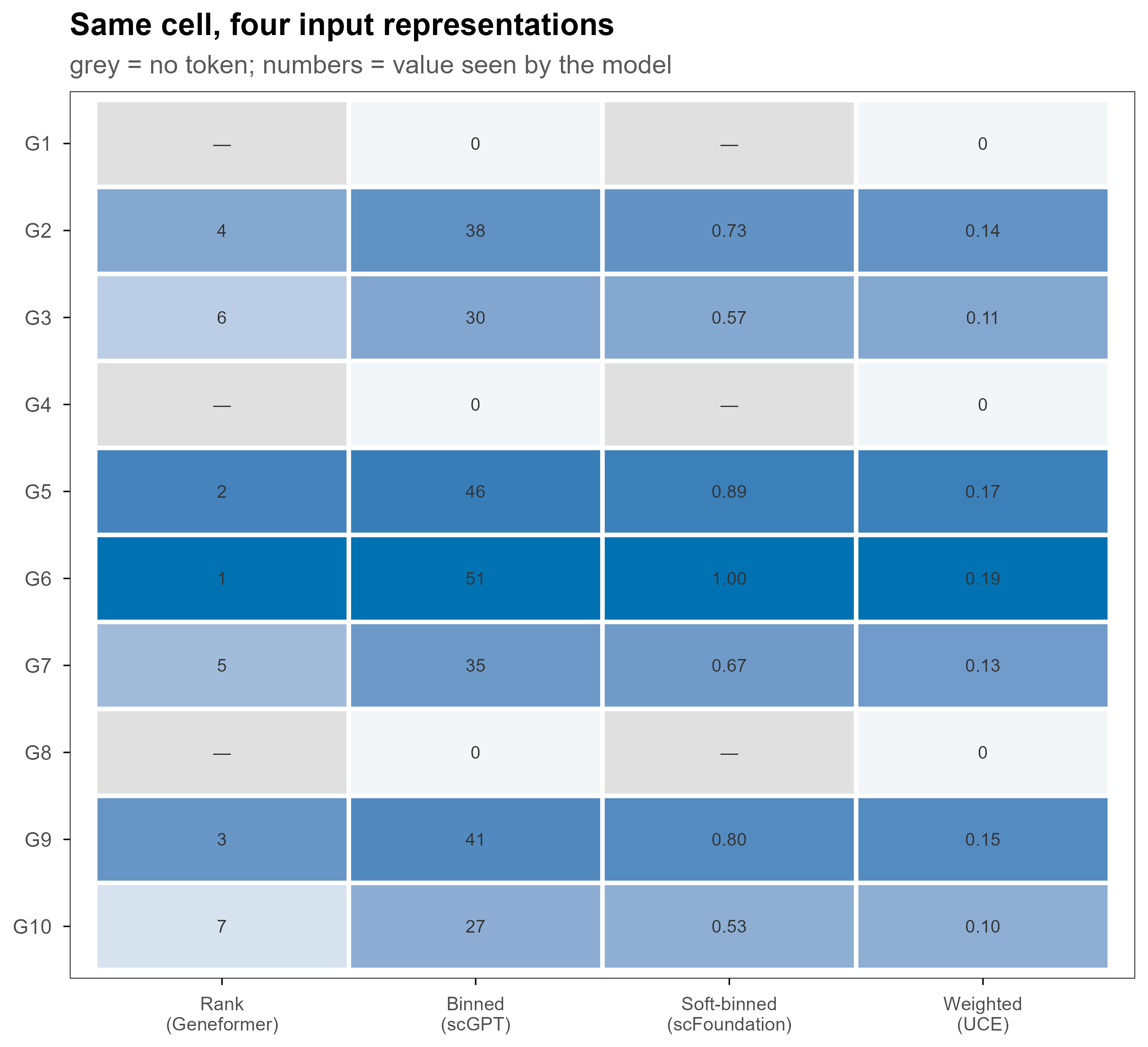
为了让四种方法可以直接对比，我们固定一个 10 基因的细胞：原始计数为

To compare the four schemes directly, we fix a single cell with ten genes; the raw counts are

genes  <- paste0("G", 1:10)
counts <- c(0, 12, 3, 0, 45, 120, 7, 0, 21, 2)
lib    <- sum(counts)
norm   <- log1p(counts / lib * 1e4)

toy <- data.frame(
  gene   = genes,
  count  = counts,
  cpt10k = round(counts / lib * 1e4, 1),
  log1p  = round(norm, 3)
)
toy

   gene count cpt10k log1p
1    G1     0    0.0 0.000
2    G2    12  571.4 6.350
3    G3     3  142.9 4.969
4    G4     0    0.0 0.000
5    G5    45 2142.9 7.670
6    G6   120 5714.3 8.651
7    G7     7  333.3 5.812
8    G8     0    0.0 0.000
9    G9    21 1000.0 6.909
10  G10     2   95.2 4.567

这段数据故意包含三个零、一个极高表达（G6 = 120）和几个低表达（G3 = 3，G10 = 2）。零值检验”是否保留零”，高表达检验”是否压缩动态范围”，低表达检验”分箱后是否被并入第一个箱”。

The toy vector deliberately contains three zeros, one very high value (G6 = 120), and several low values (G3 = 3, G10 = 2). Zeros test how the scheme handles missingness, the high value tests dynamic-range compression, and the low values test whether binning merges them into the first bin.

3. 排序编码：Geneformer / Rank-based encoding

3.1 计算过程 / The computation

Geneformer 的做法是：按细胞内表达量从高到低排序，去掉零表达基因，只保留前 \(L\) 个（V1 中 \(L = 2048\)），把每个基因的身份作为一个 token。表达量本身不进入嵌入，只决定顺序与是否入选。

Geneformer ranks genes within each cell from highest to lowest expression, drops zero-expression genes, keeps only the top \(L\) (with \(L = 2048\) in V1), and uses each gene’s identity as a token. The expression level itself never enters the embedding; it only determines the order and the cutoff.

# pseudocode: rank-based encoding
x    <- normalize_counts(counts)          # x: [G]
keep <- which(x > 0)                      # drop zeros
ord  <- keep[order(x[keep], decreasing = TRUE)]
tokens <- gene_ids[ord][1:L]              # shape [L]
input  <- gene_embedding[tokens]          # [L, D] + positional encoding

张量维度：输入是 \([B, L]\) 的整数索引，嵌入后为 \([B, L, D]\)。注意这里没有表达值嵌入：\([B, L]\) 里只有基因 ID。

Tensor shapes: the input is an integer tensor \([B, L]\), embedded to \([B, L, D]\). Note that there is no value embedding; the \([B, L]\) tensor contains gene IDs only.

3.2 信息在哪里丢失 / Where information is lost

• 绝对丰度完全丢失：把所有非零值乘以 100，得到的输入完全相同。
  Absolute abundance is lost: multiplying every non-zero value by 100 yields an identical input.
• 比值信息丢失：只要排序不变，G5 是 G3 的 15 倍还是 1.5 倍，模型看到的都一样。
  Ratios are lost: as long as the ordering is unchanged, a 15-fold versus 1.5-fold difference is invisible.
• 截断：第 2049 名之后的基因被直接丢弃，低表达但关键的调控基因可能消失。
  Truncation: genes below rank 2049 disappear, including potentially important lowly expressed regulators.
• 零值：不进入序列，因此”这个基因没表达”与”这个基因不在面板上”在输入上无法区分。
  Zeros never enter the sequence, so “not expressed” and “not on the panel” are indistinguishable.

3.3 为什么这样做有效 / Why it works

排序编码对单调变换不变（monotone invariant），因此对平台差异、测序深度差异天然鲁棒；词表只由基因 ID 组成，规模可控；序列长度固定，便于批量训练。代价是模型无法学习”剂量—效应”，这对扰动预测是一个结构性限制。

Rank encoding is invariant to monotone transformations, hence naturally robust to platform and depth differences; the vocabulary contains only gene IDs and stays manageable; sequence length is fixed, which simplifies batching. The cost is that the model cannot learn dose–response relationships, a structural limitation for perturbation prediction.

4. 分箱编码：scGPT / Binned expression encoding

4.1 计算过程 / The computation

scGPT 把连续表达值映射到固定数量的箱（默认 51 个），每个箱有独立的可学习嵌入；最终输入是基因嵌入 + 表达箱嵌入 + 位置嵌入三者之和。零值通常占用第 0 号箱，因此零值仍然是一个 token，只是携带”零”这个信息。

scGPT maps continuous expression values into a fixed number of bins (51 by default), each with its own learnable embedding; the input is the sum of gene embedding, value-bin embedding, and positional embedding. Zeros typically occupy bin 0, so a zero still produces a token that explicitly encodes “zero”.

# pseudocode: binned encoding
x      <- normalize_counts(counts)                 # [G]
bins   <- cut(x, breaks = bin_edges, labels = FALSE)  # edges from training data
keep   <- hvg_mask                                 # or all genes
tok    <- gene_ids[keep]
val    <- bins[keep]                               # [L]
input  <- gene_emb[tok] + value_emb[val] + pos_emb(seq_along(tok))  # [L, D]

4.2 信息在哪里丢失 / Where information is lost

• 箱宽：边界通常由训练集的分位数或对数范围决定；两个相差 10% 的值可能落入同一箱。
  Bin width: boundaries are usually set from training-set quantiles or log ranges; two values differing by 10% may share a bin.
• 长尾：极高表达被压到最后一个箱，箱内差异消失。
  Long tail: very high values collapse into the last bin, erasing within-bin differences.
• 零值语义：零被当作一个普通类别，模型必须自己学会”零”与”低表达”的区别。
  Zero semantics: zero becomes an ordinary category, and the model must learn the difference between “zero” and “low” by itself.
• 跨数据集：若新数据的动态范围超出训练边界，大量值会被压到首尾箱。
  Cross-dataset: if a new dataset exceeds the training range, many values pile into the edge bins.

4.3 分箱的隐含假设 / The implicit assumption

分箱假设”表达量的差异在箱的尺度上才有意义”，也就是承认测量噪声大于箱宽。这在 log 空间里通常成立，但在低表达区（0、1、2 counts）不成立：那里箱宽可能小于泊松噪声。

Binning assumes that differences matter only at the bin scale, i.e., that measurement noise exceeds the bin width. That is usually true in log space but not at low counts (0, 1, 2), where bin width can be smaller than Poisson noise.

5. 连续值编码：scFoundation 与 scPRINT / Continuous value encoding

5.1 scFoundation：软离散化 / scFoundation: soft discretization

scFoundation 的编码器只接收非零且未被掩码的基因，这是它与前两种方法最大的结构差别：序列长度随细胞变化，而不是固定的 \(L\)。表达值先做测序深度感知的归一化，再通过”自动离散化”（auto-discretization）模块转成向量：把标量投影到 100 个可学习的桶上，取其加权和，得到连续而平滑的表示。

scFoundation’s encoder consumes only non-zero, non-masked genes, a structural difference from the previous two schemes: sequence length varies per cell instead of being a fixed \(L\). Values are first normalized in a read-depth-aware way, then passed through an auto-discretization module that projects the scalar onto 100 learnable buckets and takes a weighted sum, yielding a smooth, near-continuous representation.

# pseudocode: continuous value encoding (scFoundation-style)
x     <- normalize_read_depth(counts)        # [G]
keep  <- which(x > 0 & !masked)              # variable length
v     <- x[keep] / scale                     # [n]
w     <- softmax(bucket_proj(v))             # [n, 100]
e_val <- w %*% bucket_emb                    # [n, D]
input <- gene_emb[gene_ids[keep]] + e_val    # [n, D]

它”连续”的地方在于桶的加权是软的、可微的；它仍然离散的地方在于只有 100 个基向量。严格说，这是一种学习得到的软分箱，而不是逐值独立的连续嵌入。

It is “continuous” in that bucket weights are soft and differentiable, but still discrete in having only 100 basis vectors. Strictly speaking, this is a learned soft binning, not a per-value continuous embedding.

5.2 scPRINT：连续投影 + 生物学先验 / scPRINT: continuous projection with biological priors

scPRINT 走的是另一条路：基因嵌入由蛋白质语言模型（ESM2）初始化，表达值经归一化后由一个可学习的连续投影映射为向量，再与基因嵌入相加；解码端使用零膨胀负二项（ZINB）式的似然来重建计数。这样做的结果是：表达值不被量化成箱，而是保留在连续空间中。

scPRINT takes a different route: gene embeddings are initialized from a protein language model (ESM2), normalized expression values are mapped by a learnable continuous projection, and the two are summed; the decoder reconstructs counts with a zero-inflated negative-binomial-style likelihood. Expression values therefore stay in a continuous space rather than being quantized.

需要注意：不同版本的实现细节（归一化方式、是否加入批次 token、是否使用染色体位置编码）可能不同，阅读时应以对应版本的代码为准。

Note that implementation details (normalization, batch tokens, whether chromosomal position encodings are used) differ across versions; always check the code for the version you use.

5.3 连续编码的代价 / The cost of continuity

连续值保留了剂量信息，但也把尺度问题直接交给了模型：不同平台、不同化学试剂、不同测序深度会产生系统性偏移。若训练数据足够大且多样，模型可以学到这些偏移；若目标数据集与训练分布差异较大，连续值反而会成为分布外（OOD）风险的来源。

Continuous values preserve dose information but hand the scaling problem to the model: platforms, chemistries, and depths introduce systematic shifts. With enough diverse training data the model can learn them; on a target dataset far from the training distribution, continuous values become a source of out-of-distribution risk.

6. 基因身份与生物学先验 / Gene identity and biological priors

6.1 基因词表的三种来源 / Three sources of gene identity

• 可学习词表：每个基因 ID 对应一个自由向量（Geneformer、scGPT）。灵活，但只能表示训练中出现过的基因。
  Learnable vocabulary: one free vector per gene ID (Geneformer, scGPT). Flexible, but limited to genes seen in training.
• 基因共表达先验：用 gene2vec 之类的共表达嵌入初始化（scBERT）。在数据稀少时提供归纳偏置。
  Co-expression priors: initialization from gene2vec-style embeddings (scBERT), providing inductive bias when data are scarce.
• 蛋白质语言模型：用 ESM2 的蛋白序列嵌入作为基因向量（UCE、scPRINT）。跨物种可用，且新基因只要知道序列就能编码。
  Protein language models: ESM2 sequence embeddings as gene vectors (UCE, scPRINT). Species-agnostic, and a new gene can be encoded as long as its sequence is known.

6.2 为什么这决定了”零样本”能力 / Why this determines zero-shot behaviour

如果一个模型只有可学习词表，遇到训练集里没有的基因（新组装、非模式物种、罕见 isoform），它只能退化为 <unk>。而基于蛋白序列的编码没有这个问题——这也是 UCE 能跨八个物种工作的关键原因之一。基因身份的可迁移性，往往比表达值的分辨率更能决定跨数据集表现。

If a model relies solely on a learnable vocabulary, genes absent from training (new assemblies, non-model species, rare isoforms) degrade to <unk>. Sequence-based encodings do not have this problem, which is a key reason UCE works across eight species. Transferability of gene identity often matters more for cross-dataset performance than the resolution of expression values.

7. 横向比较 / Comparative analysis

7.1 玩具数据上的四种编码 / Four encodings on the toy vector

enc <- data.frame(
  gene  = genes,
  count = counts,
  log1p = round(norm, 3)
)
enc$rank <- ifelse(norm > 0, rank(-norm, ties.method = "first"), NA)
enc$bin  <- ifelse(norm > 0,
                   pmin(findInterval(norm, seq(0, max(norm), length.out = 52)), 51),
                   0)
enc$scfound <- ifelse(norm > 0, round(norm / max(norm), 3), NA)
enc$weight  <- round(norm / sum(norm), 3)

knitr::kable(
  enc,
  col.names = c("gene", "count", "log1p", "rank (Geneformer)",
                "bin (scGPT)", "value (scFoundation)", "weight (UCE)"),
  digits = 3,
  caption = "同一组 10 个基因在四种编码下的输入。rank 为细胞内排序（NA = 被丢弃）；bin 为 51 箱离散化（0 = 零值箱）；value 为归一化后的连续值；weight 为按表达量采样的概率。"
)

同一组 10 个基因在四种编码下的输入。rank 为细胞内排序（NA = 被丢弃）；bin 为 51 箱离散化（0 = 零值箱）；value 为归一化后的连续值；weight 为按表达量采样的概率。

gene	count	log1p	rank (Geneformer)	bin (scGPT)	value (scFoundation)	weight (UCE)
G1	0	0.000	NA	0	NA	0.000
G2	12	6.350	4	38	0.734	0.141
G3	3	4.969	6	30	0.574	0.111
G4	0	0.000	NA	0	NA	0.000
G5	45	7.670	2	46	0.887	0.171
G6	120	8.651	1	51	1.000	0.193
G7	7	5.812	5	35	0.672	0.129
G8	0	0.000	NA	0	NA	0.000
G9	21	6.909	3	41	0.799	0.154
G10	2	4.567	7	27	0.528	0.102

注意两个细节：G1、G4、G8 的计数为 0，在 Geneformer 与 scFoundation 中根本不出现，在 scGPT 中作为一个 bin-0 token 出现，在 UCE 中采样概率为 0。同一个”零”，在四种方案里有四种不同的本体论地位。

Two details matter: G1, G4, and G8 have zero counts, so they do not exist as tokens in Geneformer or scFoundation, exist as bin-0 tokens in scGPT, and have zero sampling probability in UCE. The same “zero” has four different ontological statuses across the four schemes.

max_rank <- max(enc$rank, na.rm = TRUE)

plot_df <- bind_rows(
  data.frame(gene = enc$gene, method = "Rank\n(Geneformer)",
             score = ifelse(is.na(enc$rank), NA, 1 - (enc$rank - 1) / max_rank),
             label = ifelse(is.na(enc$rank), "—", as.character(enc$rank))),
  data.frame(gene = enc$gene, method = "Binned\n(scGPT)",
             score = enc$bin / 51,
             label = as.character(enc$bin)),
  data.frame(gene = enc$gene, method = "Soft-binned\n(scFoundation)",
             score = enc$scfound,
             label = ifelse(is.na(enc$scfound), "—", sprintf("%.2f", enc$scfound))),
  data.frame(gene = enc$gene, method = "Weighted\n(UCE)",
             score = enc$weight / max(enc$weight),
             label = ifelse(enc$weight == 0, "0", sprintf("%.2f", enc$weight)))
) %>%
  mutate(
    gene = factor(gene, levels = rev(enc$gene)),
    method = factor(method, levels = c("Rank\n(Geneformer)", "Binned\n(scGPT)",
                                       "Soft-binned\n(scFoundation)", "Weighted\n(UCE)"))
  )

ggplot(plot_df, aes(method, gene, fill = score)) +
  geom_tile(colour = "white", linewidth = 0.9) +
  geom_text(aes(label = label), size = 2.7, colour = "grey20") +
  scale_fill_gradient(low = "#F2F6F9", high = blog_pal[["blue"]],
                      na.value = "grey88", guide = "none") +
  labs(x = NULL, y = NULL,
       title = "Same cell, four input representations",
       subtitle = "grey = no token; numbers = value seen by the model") +
  theme(axis.text.x = element_text(size = 8, lineheight = 0.9))

Figure 1: 同一组 10 个基因在四种编码下的输入表示。颜色表示编码后数值的相对大小，灰色表示该基因在该方案中不产生 token，数字为实际进入模型的离散值或连续值。

7.2 维度与计算成本 / Dimensions and cost

设批大小为 \(B\)、序列长度为 \(L\)、隐藏维度为 \(D\)。自注意力的计算与显存都随 \(L^2\) 增长：

\[ \text{cost}_{\text{attn}} \;\propto\; B \cdot L^2 \cdot D \]

With batch size \(B\), sequence length \(L\), and hidden dimension \(D\), both compute and memory of self-attention grow as \(L^2\):

L <- seq(128, 8192, length.out = 300)
ggplot(data.frame(L = L, cost = (L / 128)^2), aes(L, cost)) +
  geom_line(colour = blog_pal[["blue"]], linewidth = 0.9) +
  geom_vline(xintercept = c(512, 2048), linetype = "dashed",
             colour = blog_pal[["vermillion"]], linewidth = 0.4) +
  annotate("text", x = 512, y = 5200, label = "512", size = 3,
           colour = blog_pal[["vermillion"]], hjust = -0.2) +
  annotate("text", x = 2048, y = 5900, label = "2048 (Geneformer)",
           size = 3, colour = blog_pal[["vermillion"]], hjust = -0.05) +
  scale_x_continuous(breaks = c(0, 2000, 4000, 6000, 8000),
                     limits = c(0, 8300)) +
  labs(x = "sequence length L (genes per cell)", y = expression("relative attention cost"~(L/128)^2),
       title = "Why sequence length dominates",
       subtitle = "quadratic scaling in self-attention")

Figure 2: 自注意力成本随序列长度的二次增长（解析曲线，未含常数因子）。Geneformer 固定 2,048；稀疏编码的有效长度随细胞非零基因数变化；分箱方案的长度等于保留的基因数。

因此，“保留所有基因”在计算上并不可行；“只保留前 2048 个”用截断换取固定成本；“只编码非零基因”用变长序列换取稀疏性；“按表达量采样固定数量基因”（UCE）则把长度变成超参数。四种策略的差别，本质上是如何花 token 预算。

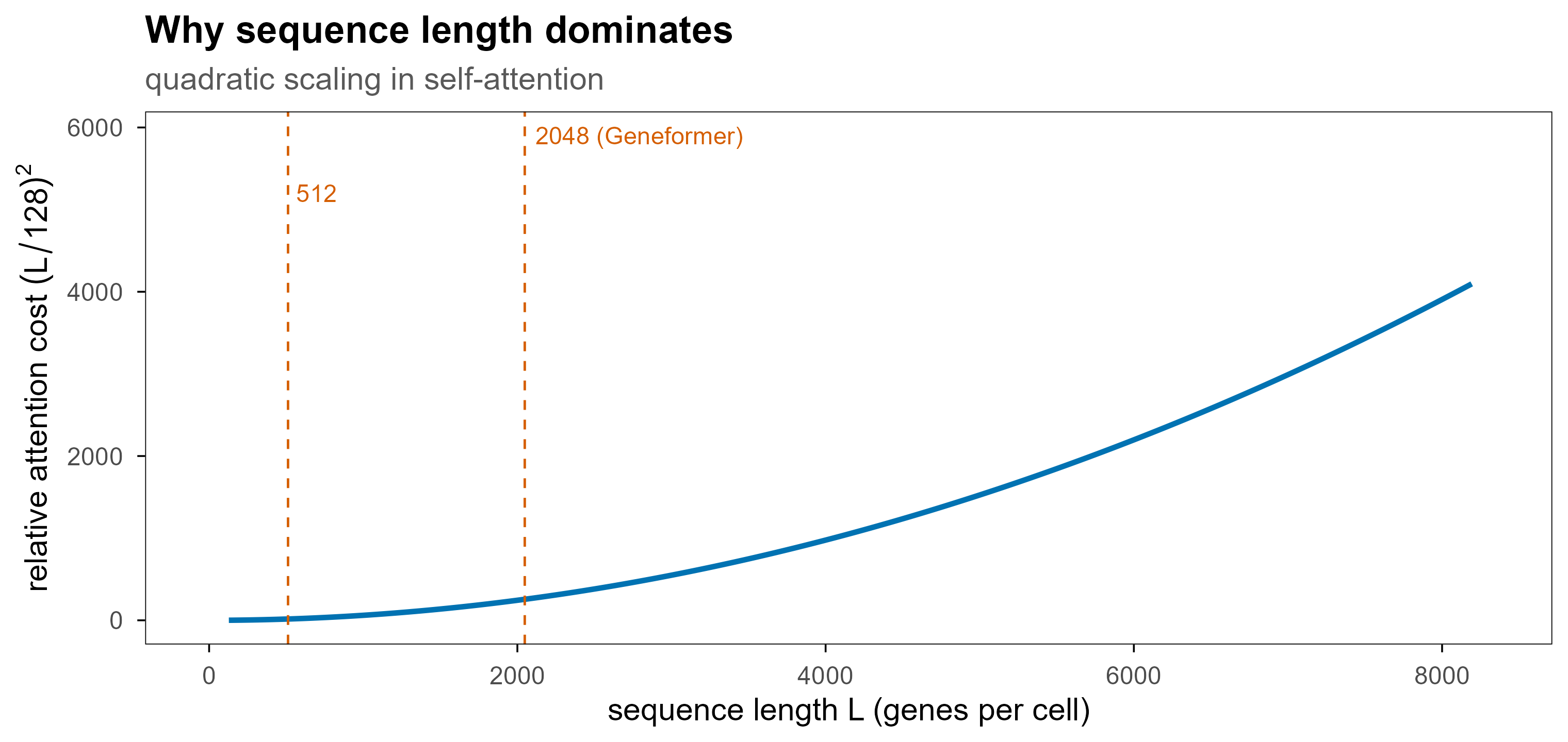
Keeping all genes is therefore computationally infeasible; keeping the top 2,048 trades truncation for fixed cost; encoding only non-zero genes trades variable length for sparsity; sampling a fixed number of genes by expression (UCE) turns length into a hyperparameter. The four strategies differ mainly in how they spend the token budget.

7.3 比较表 / Comparison table

方法 / Method	代表模型 / Models	Token 组成 / Composition	零值 / Zeros	长度 / Length	主要损失 / Main loss
Rank	Geneformer	gene ID only	丢弃 / dropped	2,048 固定	绝对量与比值
Binned	scGPT	gene + bin + pos	bin 0 token	HVG 数	箱内差异、长尾
Soft-binned	scFoundation	gene + 100 桶权重	丢弃 / dropped	非零基因数	桶数上限
Continuous	scPRINT	gene (ESM2) + 投影	单独处理	基因数	尺度依赖
Weighted	UCE	ESM2 + 采样	概率为 0	采样数	采样噪声

7.4 一个必须强调的方法论警告 / A necessary methodological caveat

不同模型在 benchmark 上的差异，不能直接归因于编码方式。架构、参数量、训练语料、预训练目标（MLM、自回归、对比学习）、下游微调策略都会混入。已有的系统评测显示，在基因扰动预测任务上，一些基础模型并未稳定超过简单的线性基线（Ahlmann-Eltze et al., 2025），这说明”模型更大、编码更复杂”并不自动等于”预测更准”。

Differences in benchmark performance cannot be attributed to the encoding scheme alone. Architecture, parameter count, training corpus, pretraining objective (MLM, autoregressive, contrastive), and fine-tuning strategy all confound the comparison. Systematic evaluations show that, for genetic perturbation prediction, some foundation models do not reliably beat simple linear baselines (Ahlmann-Eltze et al., 2025), which means “bigger model, fancier encoding” does not automatically imply “better prediction”.

8. 开放问题 / Open questions

1. 单调不变性是否是优点？ 排序编码对平台差异鲁棒，但它是否也在结构上阻止了剂量—效应学习？
   Is monotone invariance a virtue? Rank encoding is robust to platform shifts, but does it structurally prevent learning dose–response?
2. 零的语义：把零当作一个 token、直接丢弃、还是用零膨胀似然建模，哪一种最有利于扰动预测？
   Semantics of zero: token, drop, or zero-inflated likelihood — which best serves perturbation prediction?
3. 跨物种与跨平台：蛋白序列初始化的基因嵌入是否真的优于可学习词表？现有证据多来自聚类任务，缺少扰动任务的对照。
   Cross-species and cross-platform: are protein-sequence-initialized gene embeddings really better than learnable vocabularies? Most evidence comes from clustering, not perturbation.
4. 多组学：ATAC、蛋白、空间信息如何与表达值编码对齐？简单相加是否足够？
   Multi-omics: how should ATAC, protein, and spatial modalities be aligned with expression encoding? Is summation enough?
5. token 预算：在固定算力下，是”更多基因 × 更低分辨率”更好，还是”更少基因 × 更高分辨率”更好？
   Token budget: at fixed compute, is “more genes × lower resolution” better than “fewer genes × higher resolution”?

9. 对虚拟细胞模型的实用建议 / Practical recommendations

• 保留数值通道：即使主编码用 rank，也建议额外提供一个低维连续值通道（例如前 2,048 个基因的表达分位数），用于剂量相关任务。
  Keep a value channel: even with rank as the main encoding, add a low-dimensional continuous channel (e.g., expression quantiles of the top genes) for dose-sensitive tasks.
• 显式建模零：不要把零与缺失混为一谈；至少提供 expressed / not expressed 的掩码。
  Model zeros explicitly: do not conflate zero with missing; provide at least an expressed/not-expressed mask.
• 基因身份与物种解耦：优先使用序列或同源映射，避免 <unk> 在跨物种时吞掉信息。
  Decouple gene identity from species: prefer sequence or orthology mappings so that <unk> does not swallow information cross-species.
• 报告编码消融：任何声称”编码更好”的工作，都应固定架构、数据与训练目标，只改变编码。
  Report encoding ablations: any claim that an encoding is better should hold architecture, data, and objective fixed and vary only the encoding.
• 控制 token 预算：在比较不同编码时，应让总 token 数（或总算力）匹配，否则比较的是成本而非编码。
  Match the token budget: when comparing encodings, match total tokens (or compute); otherwise you compare cost, not encoding.

10. 值得测试的四个技术问题 / Four testable questions

1. 单调变换消融：在同一模型上，把输入从 rank 改为”rank + 表达值分位数”，在扰动预测任务上是否提升？若提升，说明剂量信息确实被 rank 编码丢弃了。
   Monotone-transform ablation: with the same model, replace rank input by “rank + expression quantile” and test perturbation prediction. Any gain indicates that dose information is indeed lost under rank encoding.

2. 箱数扫描：固定架构与数据，把 bin 数从 11、51、201 扫到连续值，画出”分辨率—性能”曲线，观察是否存在平台期。
   Bin sweep: with architecture and data fixed, sweep bin counts (11, 51, 201, continuous) and plot resolution versus performance to see whether a plateau exists.

3. 零处理消融：在 scGPT 式架构上比较”bin-0 token”与”直接丢弃零”两种策略，评估对零膨胀基因（如低表达转录因子）的影响。
   Zero-handling ablation: in a scGPT-style architecture, compare bin-0 tokens against dropping zeros, focusing on zero-inflated genes such as lowly expressed transcription factors.

4. 长度—分辨率权衡：在固定算力下比较”4,096 个基因 × rank”与”1,024 个基因 × 连续值”，检验在跨数据集迁移上哪一个更稳。
   Length–resolution trade-off: at fixed compute, compare “4,096 genes × rank” with “1,024 genes × continuous values” on cross-dataset transfer.

参考文献 / References

1. Theodoris, C. V., et al. (2023). Transfer learning enables predictions in network biology. Nature 618, 616–624. doi:10.1038/s41586-023-06139-9
2. Cui, H., et al. (2024). scGPT: toward building a foundation model for single-cell multi-omics using generative AI. Nature Methods 21, 1470–1480. doi:10.1038/s41592-024-02201-0
3. Hao, M., et al. (2024). Large-scale foundation model on single-cell transcriptomics. Nature Methods 21, 1481–1491. doi:10.1038/s41592-024-02305-7
4. Kalfon, J., et al. (2025). scPRINT: pre-training on 50 million cells allows robust gene network predictions. Nature Communications 16, 3607. doi:10.1038/s41467-025-58699-1
5. Yang, F., et al. (2022). scBERT as a large-scale pretrained deep language model for cell type annotation of single-cell RNA-seq data. Nature Machine Intelligence 4, 852–866. doi:10.1038/s42256-022-00534-z
6. Rosen, Y., et al. (2026). Universal cell embedding provides a foundation model for cell biology. Nature. doi:10.1038/s41586-026-10689-z
7. Ahlmann-Eltze, C., Huber, W., & Anders, S. (2025). Deep-learning-based gene perturbation effect prediction does not yet outperform simple linear baselines. Nature Methods. doi:10.1038/s41592-025-02772-6
8. Kedzierska, K. Z., et al. (2025). Zero-shot evaluation reveals limitations of single-cell foundation models. Genome Biology.
9. Zhao, H., et al. (2023). xTrimoGene: an efficient and scalable representation learner for single-cell RNA-seq data. NeurIPS 2023.
10. Geneformer official repository: https://github.com/ctheodoris/Geneformer
11. scGPT official repository: https://github.com/bowang-lab/scGPT
12. scFoundation official repository: https://github.com/biomap-research/scFoundation
13. scPRINT official repository: https://github.com/cantinilab/scPRINT

引用说明：标 DOI 的条目为已发表论文；官方仓库用于核对实现细节。模型实现随版本变化，引用前请核对对应 commit。

Citation note: entries with DOIs are published papers; official repositories were used to verify implementation details. Implementations change across versions; check the corresponding commit before citing.