本文由 AI(DeepSeek-Flash) 检索、整理并撰写,尚未经过人工逐条校对。文中的数学推导与数值例子都可以用文中的 R 代码复现;论文引用以 arXiv 编号为主,正式发表信息请以期刊页面为准。任何”更好的算子”的说法,都应当用文中第 5、6 章的标准去检验。
This article was researched and written by an AI system (DeepSeek-Flash) and has not been proofread line by line by a human. Every derivation and numeric example can be reproduced with the R code in this post; citations lean on arXiv identifiers, so check the journal record before citing. Any claim about a “better operator” should be tested against the criteria in sections 5 and 6.
生成本文所用的提示词(压缩后) / Prompt used to generate this article (condensed)
Write a bilingual, paragraph-by-paragraph long-form explainer on what an AI operator is. Start from 2 × 3 and separate three layers: the mathematical operation, the framework op, and the GPU kernel. Explain how one computation becomes a neuron, a layer, a module and an architecture. Cover matmul, activations, softmax, normalization, convolution, attention, graph aggregation and message passing. Compare CNN, Transformer, GNN and RGAT by their core computational idea, and explain why JEPA sits at a different level. Split “a better operator” into mathematical mechanism, low-level implementation and whole-system design, using FLOPs, memory, bandwidth and arithmetic intensity. End with how to design and validate a new operator, and what virtual-cell models need. Every number must come from code that actually runs.
1. 从最简单的计算开始:到底什么是算子? / Starting from the simplest computation
There are three things in that line: two inputs, one output, and the rule that turns inputs into the output. Multiplication is a function of two numbers, \(f(a,b)=ab\), with two properties that matter here: it takes several inputs and returns a new value, and it nests — \((2\times 3)+1=7\) is another computation built on top of it.
In mathematics an operator is a little more specific than a function. It originally meant something that acts on functions: the derivative operator \(D\) sends \(f(x)\) to \(f'(x)\), an integral operator sends \(f\) to \(\int f\). In finite dimensions operators collapse into matrices: \(y = Ax\) maps one vector to another. So “operator” has always carried two flavours: it is a map, and a map with structure that can be added, composed and inverted.
Deep learning borrowed the word and loosened it. In PyTorch an operator can be a matrix multiplication, an elementwise square root, a softmax, a convolution, a table lookup. What they share is not linearity but three things: an input tensor, an output tensor, and a local derivative that automatic differentiation can use.
The mathematical layer asks what properties the map has: linear, equivariant, invertible, expressive enough. The framework layer asks whether it can be composed and differentiated: how the forward pass runs, what the backward formula is, whether it supports batching and higher-order gradients. The hardware layer asks how fast it runs on a given chip: how many memory trips, how parallel it is, whether arithmetic intensity can keep the compute units fed.
The same act has three names: mathematically \(AB\), in the framework torch.matmul (dispatching to aten::mm), on the hardware a BLAS SGEMM call. Anyone claiming a new operator should first say which layer is new.
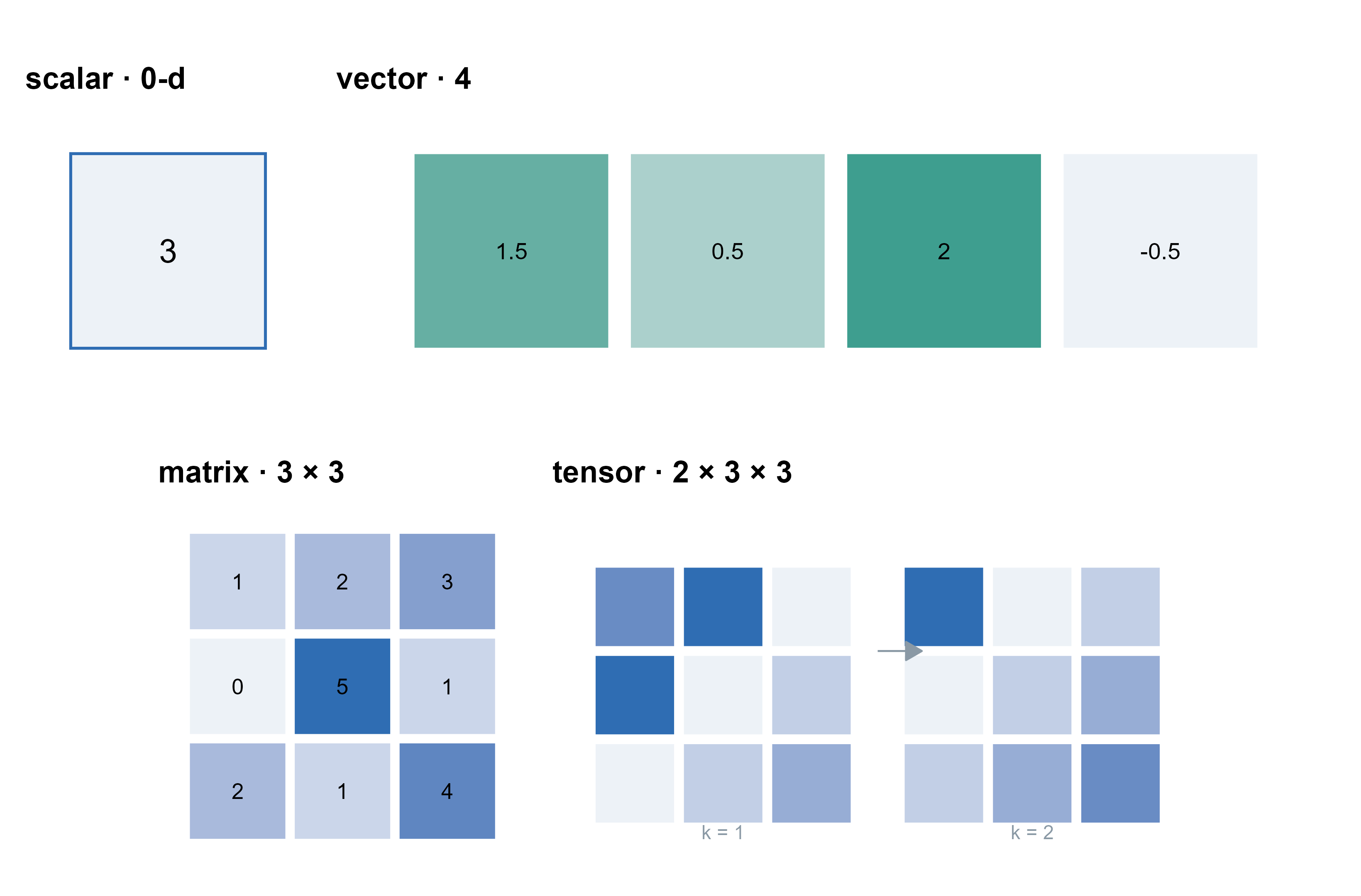
Replace “one number” by “a column of numbers” and multiplication becomes a dot product; by a 2-D array and it becomes a matrix product; keep going and you have tensor algebra. Each extra dimension buys one more kind of structure, and costs more computation.
Figure 1: 标量、向量、矩阵与三阶张量。颜色深浅表示数值大小;张量的两个切片沿第三维错开。 | Scalar, vector, matrix and a third-order tensor. Shading encodes magnitude; the two slices of the tensor are offset along the third axis.
The growth is worth memorising. Multiplying two \(n\times n\) matrices costs \(2n^3\) floating-point operations: about \(2\times 10^{9}\) at \(n=1000\), already a respectable scientific computation, and \(1.4\times 10^{11}\) at \(n=4096\). That is why one operator, matrix multiplication, has been optimised for decades: it dominates the cost of most models.
1.4 为什么算子必须”知道自己怎么求导” / Why an operator must know its own derivative
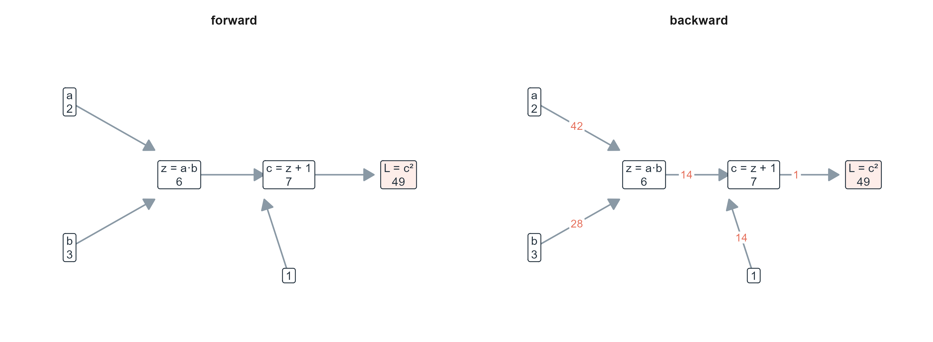
The biggest difference from classical numerics is not speed but that every step remembers its local derivative. That is the computation graph: each node is an operator, each edge a data flow; backpropagation walks the edges backwards, and each operator only has to multiply the incoming gradient by its own local derivative.
Figure 2: 一个乘法的计算图。左:前向,值沿箭头流动;右:反向,梯度沿原路返回。乘法的局部导数是另一个输入,所以 ∂L/∂a = 14×3 = 42。 | Computation graph for one multiplication. Left: forward, values flow along the arrows. Right: backward, gradients return the same way. The local derivative of a product is the other input, so ∂L/∂a = 14×3 = 42.
The easily missed point: the backward pass of a product uses the other input. Since \(\partial z/\partial a = b\), an operator’s design is not only “how to compute forward” but “which forward values must be kept so backward is possible”. That decision decides memory use — which is where FlashAttention comes back in section 5.
2. 一次计算如何变成一个神经元? / How one computation becomes a neuron
2.1 从 \(wx\) 到 \(\sigma(wx+b)\) / From \(wx\) to \(\sigma(wx+b)\)
A linear model is one multiplication: \(y = wx\). Its limitation is immediate — double the input and the output doubles; whatever \(x\) is, the output can only move along a straight line. Adding a bias \(b\) shifts that line, and it is still a line.
神经元做了两件事:先把多个输入加权求和,再用一个非线性函数 \(\sigma\) 把结果折一下:
A neuron does two things: it weighted-sums several inputs, then bends the result through a nonlinearity \(\sigma\):
\[z = \sum_{i=1}^{n} w_i x_i + b = \mathbf{w}^\top \mathbf{x} + b, \qquad y = \sigma(z)\]
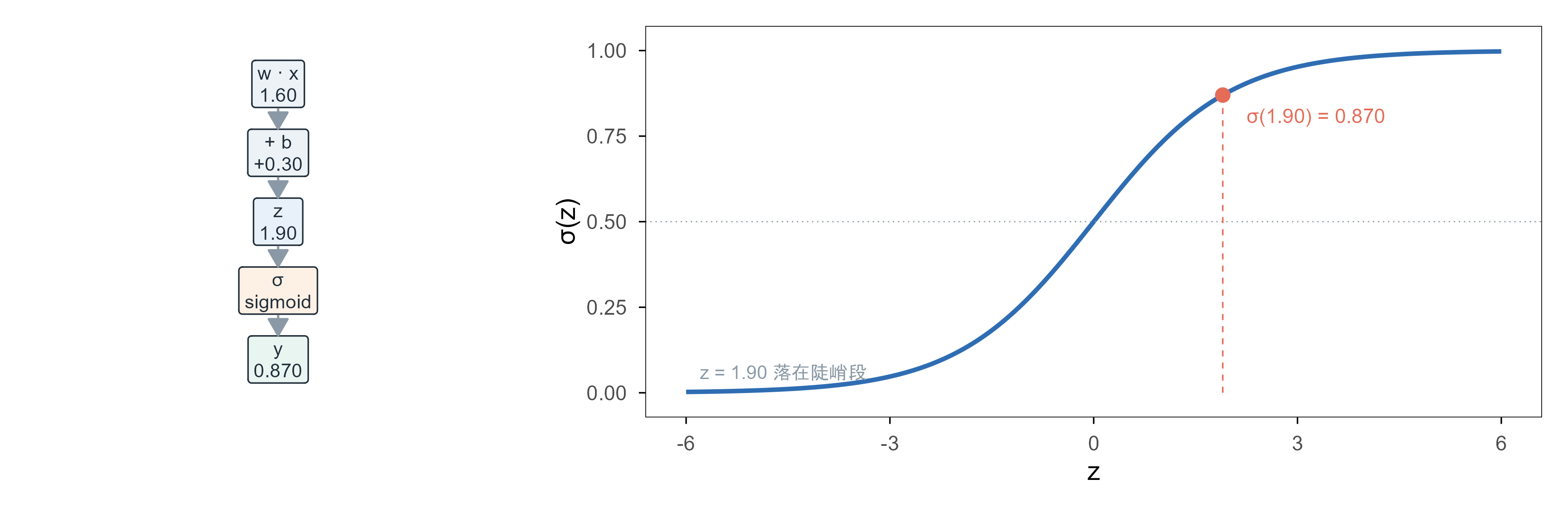
Here \(\mathbf{w}^\top\mathbf{x}\) is a dot product, one primitive operator; \(+b\) is a second; \(\sigma\) is a third. Only the three together make a “neuron”. In other words, a neuron is not an operator but a small module built from three operators in series.
Figure 3: 一个神经元的运算分解。左:三次算子调用;右:sigmoid 把 z = 1.90 折成 0.870。数字由下方代码实际算出。 | Decomposing one neuron. Left: three operator calls in series. Right: sigmoid folds z = 1.90 into 0.870. Numbers come from the code below.
Put \(n\) neurons side by side, all looking at the same input, and you get a layer: \(y=\sigma(Wx+b)\) with \(W\) an \(n\times d\) matrix. In a framework that layer is an object (nn.Linear plus an activation), but computationally it is still one matrix product, one elementwise add and one elementwise nonlinearity.
层再堆起来就是模块与架构。这三者的区别,不在于用了多少个算子,而在于信息以什么方式在元素之间流动:
Stacking layers gives modules and architectures. The difference between them is not how many operators are used, but how information moves between elements:
层(layer):一次固定的映射,输入输出形状已知。 Layer: one fixed mapping with a known input and output shape.
模块(module):几个层按固定方式组合,对外仍是一个可调用的对象,例如一个残差块、一个注意力头。 Module: several layers wired in a fixed pattern, still callable as one object — a residual block, an attention head.
架构(architecture):模块的重复方式 + 数据在序列/图/网格上的流转规则,例如”重复 12 个相同模块,每个模块里先自注意力再三层感知机”。 Architecture: how modules repeat and how data flows across a sequence, a graph or a grid — say, twelve identical blocks, each doing self-attention then an MLP.
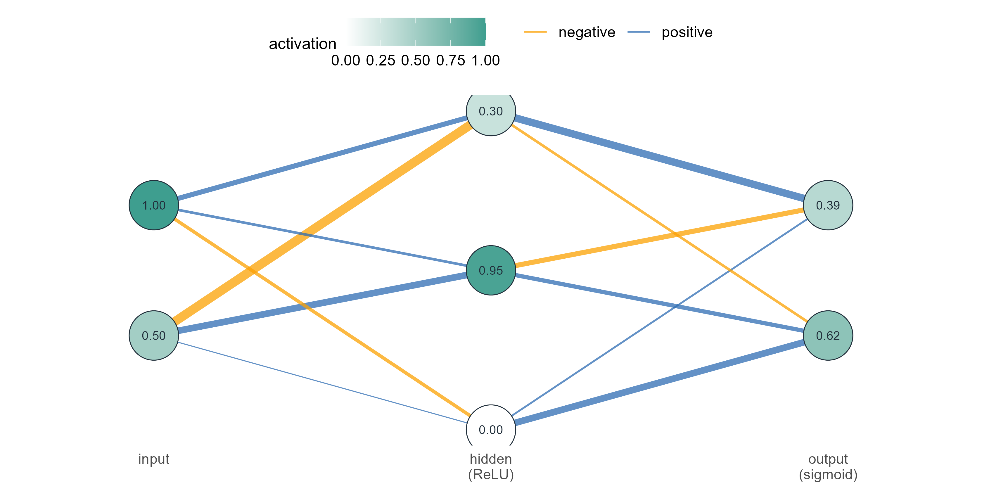
Figure 4: 一个 2-3-2 网络的前向传播。节点颜色是激活值,边宽是权重绝对值,蓝为正值、橙为负值;数字是这一组权重的真实输出。 | Forward pass through a 2-3-2 network. Node colour is activation, edge width is |weight|, blue positive and orange negative; numbers are the actual outputs for this weight set.
Four levels appear at once: operators (multiply, add, ReLU, sigmoid), layers (two linear maps), the module (the whole 2-3-2 net) and the architecture (feed-forward, layer by layer, no back edges, no cross-element links). “A 2-3-2 network” describes the architecture; “a ReLU network” describes the operator choice; “this layer has nine parameters” describes the module.
3. 现代 AI 常见的算子 / The operators modern AI is built from
3.1 矩阵乘法:一切的底座 / Matrix multiplication, the substrate
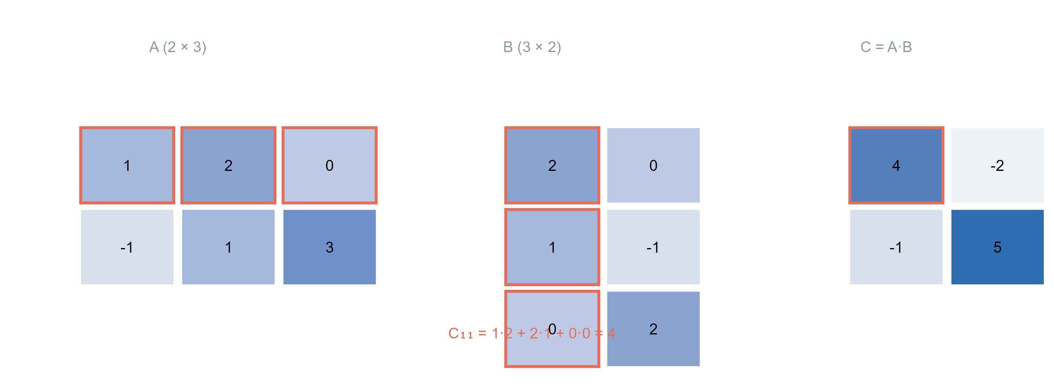
It is the inner product of one row with one column: entry \((i,j)\) of \(C\) is row \(i\) of \(A\) multiplied elementwise with column \(j\) of \(B\), then summed. Its importance is not mathematical sophistication — three nested loops describe it — but that almost everything else can be expressed through it: a dense layer is one, a convolution can be unrolled into one, and the two heavy steps inside attention are two.
Figure 5: 2 × 3 与 3 × 2 的矩阵乘法。高亮的是 C₁₁ 的计算:A 的第一行与 B 的第一列逐个相乘再相加,得到 4。 | A 2 × 3 times a 3 × 2 matrix. The highlighted entries show how C₁₁ is built: the first row of A times the first column of B, summed to 4.
The cost is \(2mnk\): two \(d\times d\) matrices need \(2d^3\). That is why the cost of a large model can almost always be summarised as parameters × tokens × layers, and every term hides a matrix multiplication.
3.2 激活函数:给线性叠加折一道弯 / Activations, bending the linear stack
Without nonlinearity, any stack collapses into one layer: \(W_2(W_1x)=(W_2W_1)x\). Activations are the only thing that breaks that identity, so a pointwise function ends up determining what the whole network can represent.
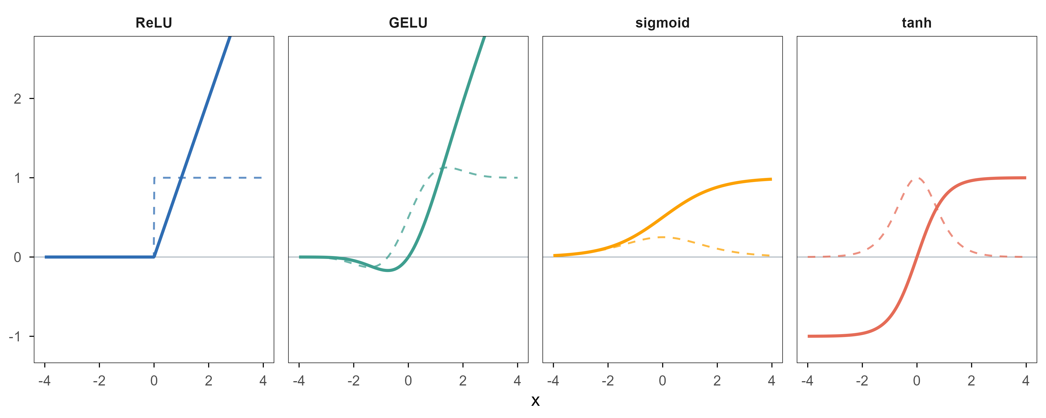
xs <-seq(-4, 4, length.out =400)relu <-pmax(0, xs)gelu <-0.5* xs * (1+tanh(sqrt(2/ pi) * (xs +0.044715* xs^3)))sig <-plogis(xs)tanhx <-tanh(xs)drelu <-as.numeric(xs >0)dgelu <-0.5* (1+tanh(sqrt(2/ pi) * (xs +0.044715* xs^3))) +0.5* xs * (1-tanh(sqrt(2/ pi) * (xs +0.044715* xs^3))^2) *sqrt(2/ pi) * (1+3*0.044715* xs^2)dsig <- sig * (1- sig)dtanh <-1- tanhx^2fns <-rbind(data.frame(x = xs, y = relu, d = drelu, name ="ReLU"),data.frame(x = xs, y = gelu, d = dgelu, name ="GELU"),data.frame(x = xs, y = sig, d = dsig, name ="sigmoid"),data.frame(x = xs, y = tanhx, d = dtanh, name ="tanh"))fns$name <-factor(fns$name, levels =c("ReLU", "GELU", "sigmoid", "tanh"))ggplot(fns) +geom_hline(yintercept =0, linewidth =0.2, colour = op_pal[["grey"]]) +geom_line(aes(x, y, colour = name), linewidth =0.9) +geom_line(aes(x, d, colour = name), linewidth =0.55, linetype ="dashed", alpha =0.75) +facet_wrap(~name, nrow =1) +scale_colour_manual(values =unname(op_pal[c("blue", "teal", "orange", "coral")]),guide ="none") +labs(x ="x", y =NULL) +coord_cartesian(ylim =c(-1.15, 2.6))
Figure 6: 四种激活函数(实线)与它们的导数(虚线)。ReLU 在 0 处不可导、导数只有 0 和 1 两个值;GELU 平滑但计算更贵;sigmoid 与 tanh 两端饱和,梯度会趋近 0。 | Four activations (solid) and their derivatives (dashed). ReLU is non-differentiable at 0 and its derivative only takes 0 or 1; GELU is smooth but costlier; sigmoid and tanh saturate, so gradients vanish.
Three practical readings. ReLU’s derivative is 0 or 1, so gradients either pass through unchanged or die, which makes it fast and makes dead units possible. GELU is smooth near zero and keeps a small negative lobe, so the gradient is more continuous, at the price of a tanh or erf. Sigmoid and tanh flatten at both ends, so gradients shrink layer by layer — one direct reason deep networks were hard to train before the 2010s.
3.3 Softmax:把分数变成分配 / Softmax, turning scores into a budget
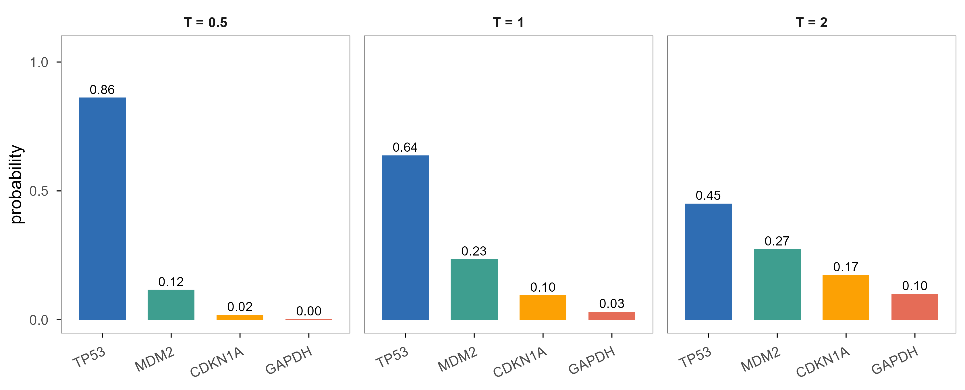
It normalises and exaggerates: outputs are positive and sum to one; a smaller temperature \(T\) makes the distribution sharper (approaching one-hot as \(T\to0\)), a larger one flattens it. Real implementations subtract the maximum before exponentiating to avoid overflow — an operator-level trick that is mathematically identical and numerically different.
Figure 7: 同一组 logits 在三个温度下的 softmax。T = 0.5 时最大的类别拿到 0.86,T = 2 时降到 0.45,分布明显变平。 | The same logits under three temperatures. At T = 0.5 the top class takes 0.86; at T = 2 it drops to 0.45 and the distribution flattens.
注意 y 轴上限是 1:每个面板里四根柱子加起来都等于 1,变化的只是”这份预算怎么分”。
Note the y axis tops out at 1: in every panel the four bars sum to 1, and only the split changes.
3.4 归一化:让数值待在可训练的区间 / Normalisation, keeping numbers in a trainable range
Normalisation is not cosmetic; it keeps the scale of each layer’s input under control, so one learning rate works everywhere. BatchNorm uses batch statistics and therefore depends on the other samples in the batch; LayerNorm normalises within one sample’s feature vector, so it is batch-size independent — the reason Transformers train stably with small batches. RMSNorm drops the mean subtraction and the bias, dividing only by the root mean square, which is cheaper.
3.5 卷积:把”邻居”写进结构 / Convolution, baking locality into the structure
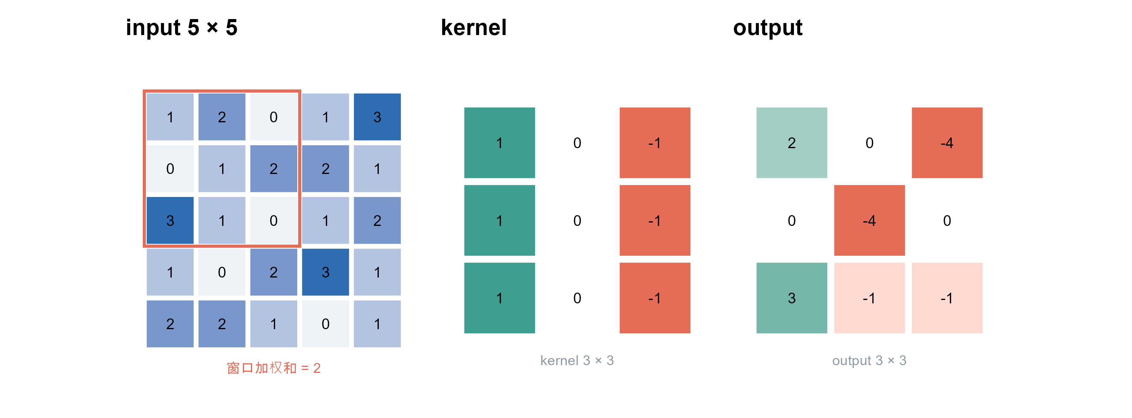
A convolution is a local weighted sum with the same small kernel sliding everywhere. Two free benefits follow: the parameter count is independent of image size (a 3×3 kernel always has nine weights), and the operator is translation-equivariant (shift the input by one pixel and the output shifts by one). The cost is a limited receptive field: one layer sees 3×3, and depth or pooling is needed to see further.
Figure 8: 5 × 5 输入与 3 × 3 核做一次卷积。左侧红框是第一个输出位置对应的窗口,右侧是完整的 3 × 3 输出,数字由代码逐个算出。 | A 3 × 3 kernel over a 5 × 5 input. The red box is the window for the first output; the right panel is the full 3 × 3 output, every entry computed by the code.
The kernel here is a vertical edge detector: a zero column in the middle, added on the left and subtracted on the right, so the output is positive where the left side is brighter than the right. Kernels are not magic; each is learning which weighted comparison to make at this position.
3.6 注意力:让任意两个位置直接对话 / Attention, letting any two positions talk
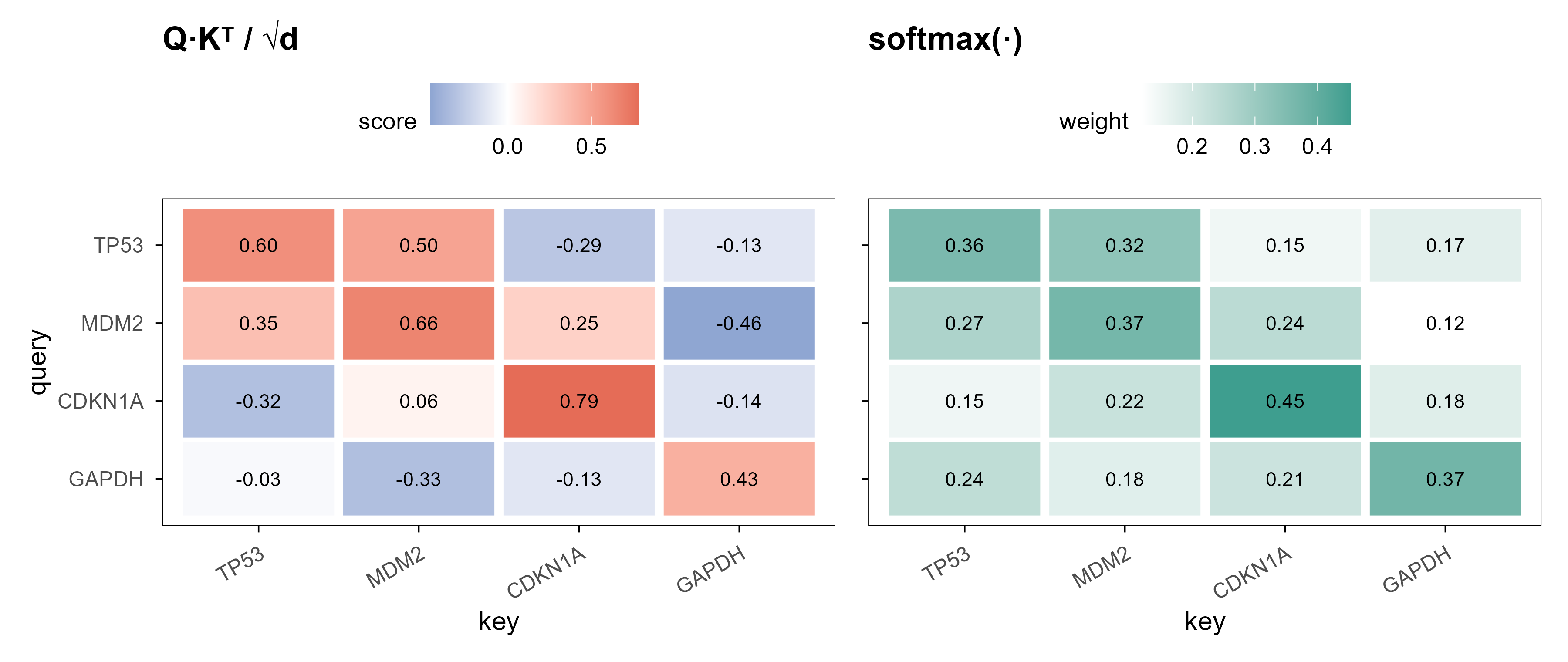
把每个 token 变成三个向量:Query(我在找什么)、Key(我是什么)、Value(我能提供什么)。\(QK^\top\) 算出所有位置两两之间的分数,除以 \(\sqrt{d_k}\) 是防止点积随维度变大而爆炸,softmax 把分数变成权重,最后用权重对 Value 加权求和。注意力的本质是一次”内容寻址”的加权平均,与卷积最大的区别是:权重不是固定的核,而是由数据自己算出来的。
Each token becomes three vectors: Query (what I am looking for), Key (what I am), Value (what I can offer). \(QK^\top\) scores every pair of positions, dividing by \(\sqrt{d_k}\) keeps dot products from exploding with dimension, softmax turns scores into weights, and the output is a weighted sum of Values. Attention is content-addressed averaging: unlike convolution, the weights are not a fixed kernel but are computed from the data.
Each row on the right is one token’s attention budget: TP53 keeps most weight on itself while MDM2 clearly looks toward CDKN1A. This who-looks-at-whom matrix is the most direct evidence when comparing Transformers with convolutions later.
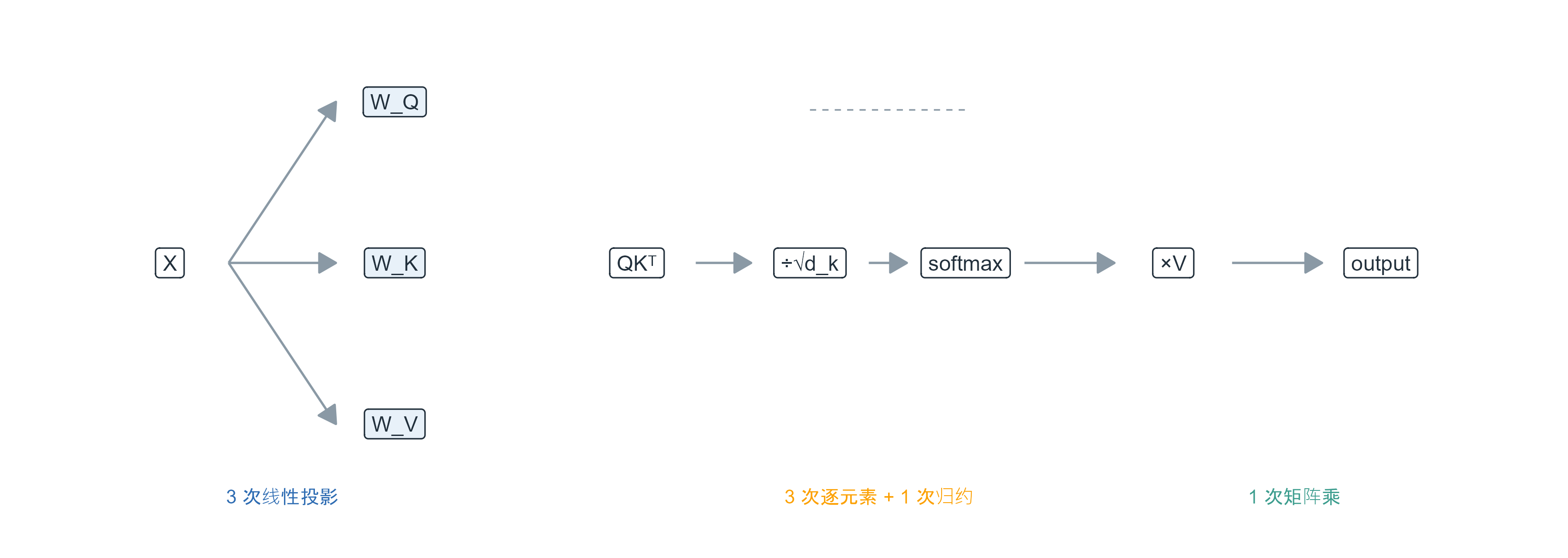
Figure 10: 注意力不是一个算子,而是至少六个算子组成的模块。每个框在框架里都对应一个 aten op;箭头是张量,不是数据流之外的魔法。 | Attention is not one operator but a module of at least six. Every box is an aten op in a framework; the arrows are tensors, nothing more.
This decomposition underpins sections 5 and 6. “FlashAttention is a new operator” and “attention is an operator” are not statements about the same layer: the former changes how these boxes exchange data, the latter is about the boxes themselves.
3.7 图聚合与消息传递:在邻居之间传纸条 / Graph aggregation and message passing
图上的节点没有固定顺序,因此合适的算子必须对邻居排列不敏感。最基础的形式是:
Graph nodes have no canonical order, so the operator must be insensitive to how neighbours are permuted. The basic form is:
\(\psi\) builds the message from \(j\) to \(i\), \(\bigoplus\) is a permutation-invariant aggregation (sum, mean, max), and \(\phi\) updates the centre. Choosing sum versus mean is already a different inductive bias: sum keeps degree information, mean normalises it away.
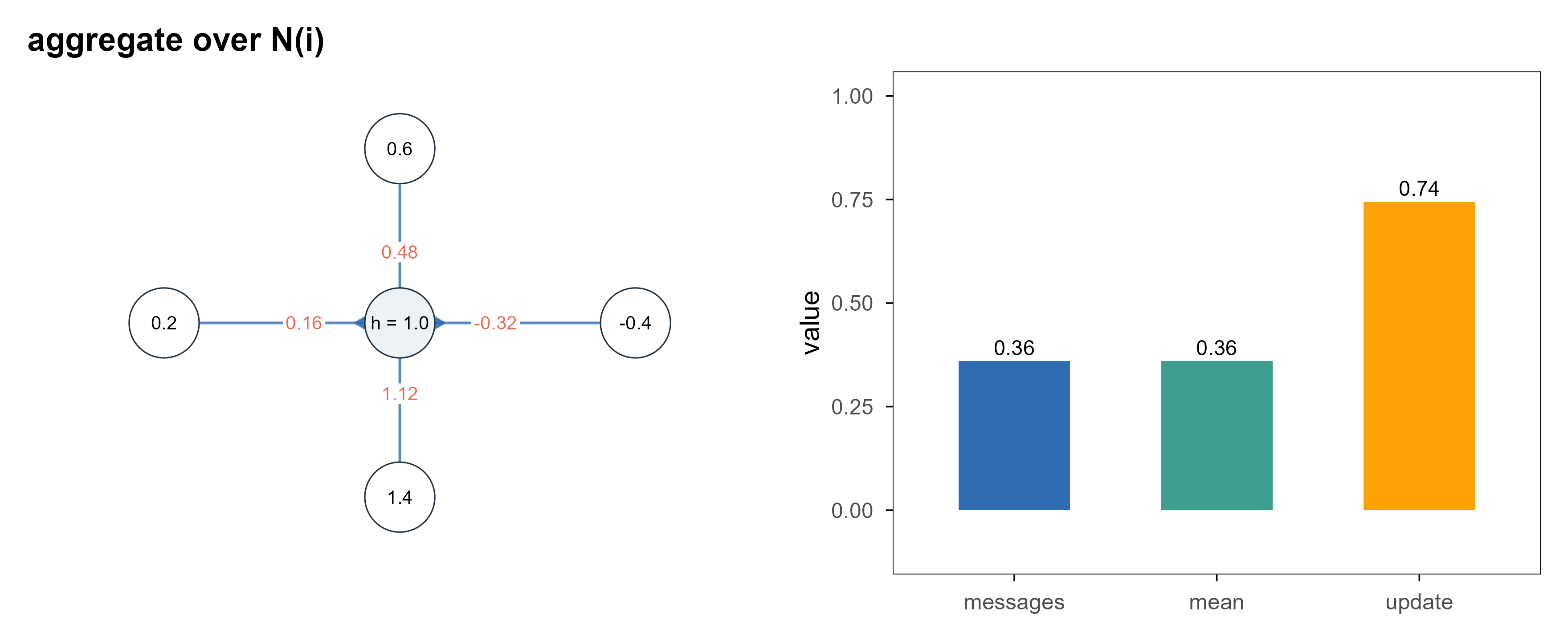
Figure 11: 一个节点的邻域聚合。四个邻居各发一条消息,聚合(这里是均值)后与中心节点自身状态一起更新。数字是这一步的真实计算结果。 | Neighbourhood aggregation for one node. Four neighbours send messages; after aggregation (mean here) the centre is updated together with its own state. Numbers are the actual result of this step.
3.8 基础算子与复合模块 / Primitives versus composite modules
把上面几种放在一起,会看到一个明显的分层:有些东西在框架里就是一个 op(加法、乘法、exp、max),有些则是一串 op 的组合,只不过被包成了一个有名字的模块。
Putting them together reveals a clear split: some things are a single op in a framework (add, multiply, exp, max), while others are chains of ops packaged under one name.
The “Params” column matters: matmul, ReLU and softmax have no trainable parameters; they are fixed rules of information processing. Convolution, attention and aggregation do have parameters; they learn how to process. Most “new operator” work is about how to parameterise this second group.
4. 为什么不同的神经网络使用不同的算子? / Why different networks need different operators
The previous sections treated operators as parts. But real networks are not random piles of parts: CNNs, Transformers and GNNs look different because they make different assumptions about what the data is shaped like. The formal name for such an assumption is an inductive bias. Put differently: an operator decides who may exchange information with whom, and by which rule; an architecture is a way of composing those rules.
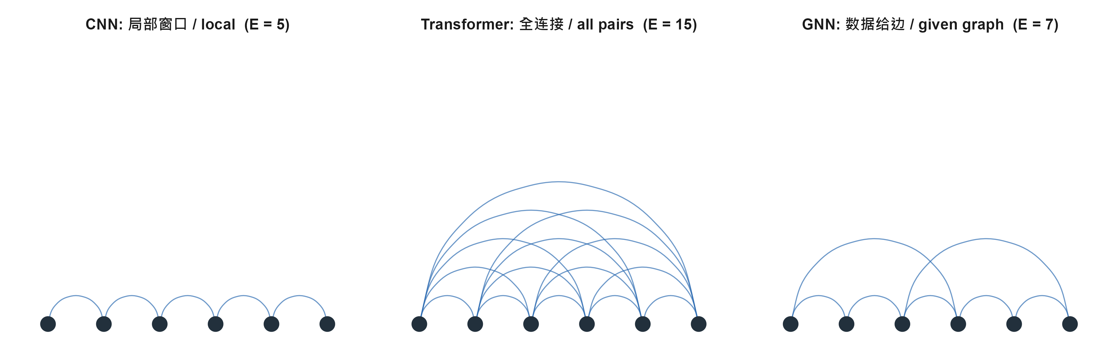
Figure 12: 同一串 6 个位置,三种「谁能和谁说话」的约定。CNN 只让相邻位置相连(3 个位置的窗口),Transformer 让所有位置两两相连,GNN 的边由数据给定。括号里是这一层的边数。 | The same six positions under three different rules about who may talk to whom. A CNN connects only neighbours (window of 3), a Transformer connects every pair, and a GNN takes its edges from the data. The brackets give the edge count of that layer.
The three panels have the same nodes and could be given the same parameter budget, yet the graph of information flow differs completely. That is the backbone of this chapter: every architecture below is just a different answer to “where does this graph come from”.
4.1 CNN:结构直接告诉你谁是邻居 / The structure tells you who the neighbours are
An image has a built-in property: nearby pixels are correlated, distant ones less so. Convolution writes that prior straight into the operator — each layer connects only a \(k\times k\) neighbourhood, and the same weights slide across the whole image:
The subscript of \(w\) is the relative offset \(j-i\), not the absolute position. So the whole image shares \(k^2\) weights instead of learning one set per location. That is weight sharing, and the property it buys is translation equivariance: shift the image and the output shifts with it, content unchanged.
The cost is equally clear: one convolution only sees neighbours. After \(L\) layers of \(k\times k\) convolution, the range a single output can see — the receptive field — is
With \(k=3\), \(L=1,3,10\) gives \(3,7,21\). To let two things 100 pixels apart interact directly you either stack 50 layers or change the operator. Depth in a CNN is not an aesthetic choice; it is the price of growing the receptive field.
4.2 Transformer:不预设邻居,让内容自己决定 / No preset neighbours, content decides
A Transformer does the opposite: it does not assume who is next to whom. Every position scores its relation to every other position and takes a weighted sum (section 3.6 already computed one). So the adjacency is not a hyperparameter; it is recomputed from the content on every forward pass. This is usually called content-based addressing.
Two consequences follow. First, any two positions are one hop apart, so long-range dependencies need no depth. Second, the operator itself is blind to input order — permute the sentence and the output permutes with it. That is permutation equivariance: \(\mathrm{Attn}(P H) = P\,\mathrm{Attn}(H)\) for any permutation matrix \(P\). Order has to be injected separately by positional encoding; that is the price of the freedom.
The third consequence is the practical one: cost. Pairing \(n\) positions gives an \(n\times n\) score matrix, \(O(n^2 d)\) compute and \(O(n^2)\) memory. Going from 1k to 32k tokens multiplies the \(n^2\) term by 1000. FlashAttention, in section 5, targets exactly the memory traffic that this \(n^2\) creates.
4.3 GNN:邻居由数据给出 / The data supplies the neighbours
Graph data is neither a grid nor fully connected: in a molecule an atom bonds only with a few others; in a cell a gene is regulated by a few others. The adjacency \(A\) is part of the input, not a hyperparameter of the model. The operator therefore has to be written as “sum along the edges”:
Because graph nodes have no canonical numbering, the aggregation \(\bigoplus\) must be permutation invariant: sum, mean and max all qualify; concatenation in a fixed order does not. The example in section 3.7 used the mean.
The main trouble with GNNs is over-smoothing: each aggregation pulls neighbouring representations closer, so with many layers all node vectors converge and separability drops. Empirically 2–4 layers is often best, which contradicts the CNN intuition that deeper is better. The reason is the same one: change the geometry of the operator and you change what depth buys you.
4.4 RGAT:边不仅有方向,还有类型 / Edges have types, not just directions
现实中的图往往带关系标签:基因 A 激活基因 B、药物 C 抑制蛋白 D、蛋白 E 与蛋白 F 形成复合物。“激活”和”抑制”是两种完全不同的信息,如果把它们压进同一个权重矩阵,模型就只能学到两者的平均值。
Real graphs usually carry relation labels: gene A activates gene B, drug C inhibits protein D, protein E forms a complex with protein F. “Activates” and “inhibits” are different kinds of information; collapsing both into one weight matrix forces the model to learn their average.
关系图注意力网络(RGAT)的做法很直接:每种关系一套参数、一套注意力。
Relational graph attention networks (RGAT) take the direct route: one set of parameters and one attention distribution per relation.
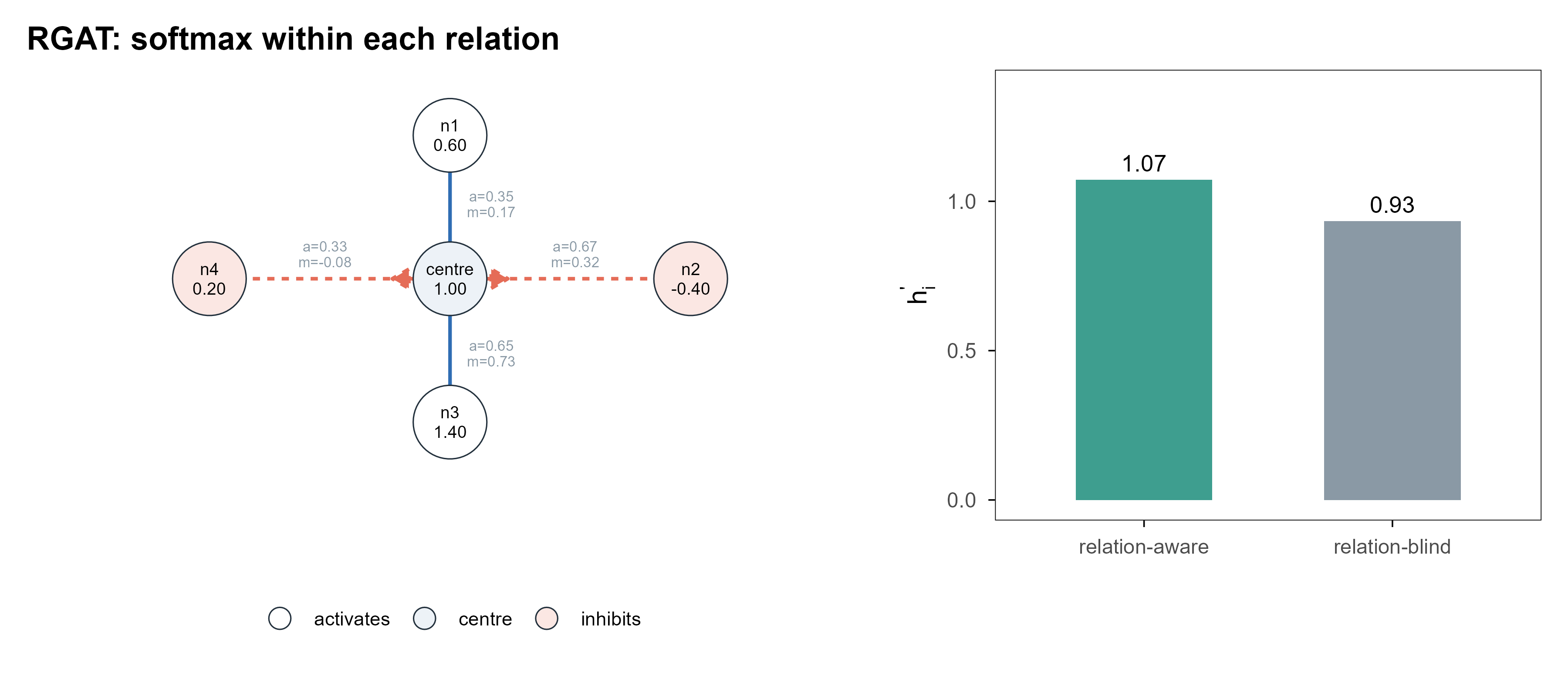
Two details matter. First, the softmax runs within each relation, not across all neighbours; otherwise a node with many activating neighbours would crowd out its inhibiting ones. Second, \(W_r\) lets the same input value produce different messages under different relations.
Figure 13: 关系感知的聚合。左侧:中心节点有 2 个激活邻居、2 个抑制邻居,每种关系各自做 softmax(括号里是注意力权重与它发出的消息)。右侧:同一个邻域,如果忽略关系类型、只做一次 softmax,得到的聚合值明显不同。 | Relation-aware aggregation. Left: two activating and two inhibiting neighbours, each relation running its own softmax (the brackets give the attention weight and the message it sends). Right: the same neighbourhood with relations ignored and a single softmax — a visibly different aggregate.
The same numbers read two ways give \(\hat h_i'=1.07\) (relation-aware) and \(0.93\) (relation-blind). The gap is modest but the direction is right: in the second version inhibiting neighbours are treated as ordinary ones, so their negative sign lives in the value but not in the structure.
RGAT belongs to the “first kind of better” (section 5): it changes the information-processing mechanism, not the implementation. The criterion is whether its expressiveness and inductive bias match the task, and the cost is again parameters: with many relations, \(|\mathcal{R}|\) weight matrices blow up, so practice often writes \(W_r\) as a linear combination of a few basis matrices.
4.5 JEPA:它不是算子,是另一层的东西 / JEPA is a different level, not an operator
A clarification is needed here. I-JEPA and V-JEPA are often mentioned alongside attention and convolution, but they answer a different question.
Attention 回答”信息怎么在位置之间流动”,JEPA 回答”模型应该预测什么、在哪里算误差”。 I-JEPA 的做法是:遮住图像的一部分块,用一个上下文编码器处理可见块,去预测被遮住块在表示空间里的向量;目标向量由另一个指数滑动平均(EMA)的编码器产生,只对预测端回传梯度。它不重建像素,因此在表示空间里算损失。类比一下:反向传播不是算子,而是训练算法;JEPA 同理,是一种自监督训练目标加一套非对称的编码器安排。它内部用的算子仍然是 ViT 的注意力和 MLP。
Attention answers “how does information flow between positions”; JEPA answers “what should the model predict, and where is the loss taken”. I-JEPA masks part of the image, encodes the visible part, and predicts the representation of the masked part; the target comes from an exponential-moving-average encoder, and gradients flow only through the prediction side. It never reconstructs pixels, so the loss lives in representation space. The analogy: backpropagation is not an operator but a training algorithm; JEPA is a self-supervised objective plus an asymmetric encoder arrangement. The operators inside it are still the ViT’s attention and MLPs.
So “JEPA is an operator” slides to the wrong level, exactly like “a Transformer is an operator”. It is better described as a representation-learning framework trained with predictive self-supervision; to discuss its computation you still return to attention, LayerNorm and matmul. The hierarchy in section 8 settles this once and for all.
The most important column is “where adjacency comes from”. It determines what the operator can express, how much data it needs, and where it fails. Changing the architecture is mostly changing the adjacency assumption; changing the operator is changing how you aggregate on that adjacency. The two are related, but they are not the same thing.
4.7 每种架构现在到底在做什么 / What each architecture actually does today
Talking about inductive bias in the abstract goes empty quickly. The table below grounds each architecture in concrete tasks, concrete systems and concrete inputs and outputs. They are chosen not because they are the most famous, but because together they show that the same task family has been solved by different architectures, and the difference comes down to the shape of the data.
架构
具体任务
代表系统
为什么是这种算子
CNN
医学影像分割:CT/MRI 中的器官、病灶、细胞核
nnU-Net
组织纹理是局部模式,同一套卷积核可以滑过整幅图;平移等变省参数
CNN
DNA 序列上的调控信号:转录因子结合位点、ChIP-seq 覆盖度
BPNet
motif 只有十几 bp,出现位置不固定,正是”局部 + 共享权重”擅长的事
Transformer
蛋白序列语言模型,输出用于变体效应预测、结构建模
ESM-2;AlphaFold2 的 Evoformer
残基之间的共变是长程的,任意两位需要直接交互,而不是叠 50 层卷积
Transformer
单细胞表达谱:细胞类型注释、扰动响应预测
scGPT、Geneformer
基因没有天然顺序和固定邻接,“看哪些基因”必须由内容决定
Transformer
语音识别、图像分类
Whisper、ViT
同一套”全对全 + 内容寻址”可以跨模态复用,代价是数据和算力
GNN
分子性质与生物活性预测
GIN、GINE(OGB 的 molhiv、molpcba 基准)
原子和化学键本来就是图;预测结果必须与原子编号无关
GNN
蛋白–配体结合构象;空间转录组的区域划分
EquiBind、DiffDock;GraphST
3D 邻接或空间邻接直接就是边,不需要”学”出来
RGAT
知识图谱补全、药物重定位、逆合成
R-GCN、RGAT(FB15k-237、WN18RR);Hetionet
边的类型带语义:“治疗”“导致”“结合”不是同一件事,压成一种边就丢了信息
JEPA
自监督预训练目标(图像、视频)
I-JEPA、V-JEPA
不是算子:它规定”在表示空间预测什么、在哪里算损失”,内部仍是 attention 与 MLP
English
Model
Concrete task
Representative system
Why this operator
CNN
Medical image segmentation: organs, lesions, nuclei in CT/MRI
nnU-Net
Tissue texture is a local pattern, so one kernel can slide over the whole image; translation equivariance saves parameters
CNN
Regulatory signal from DNA: transcription-factor binding, ChIP-seq coverage
BPNet
A motif spans ~10 bp and can appear anywhere — exactly the “local + shared weights” case
Transformer
Protein language models, used downstream for variant effects and structure
ESM-2; the Evoformer in AlphaFold2
Co-variation between residues is long-range; any two positions need direct interaction instead of 50 stacked convolutions
The thing worth noticing is that many of these tasks are done by everyone. Image classification was done by ResNet and by ViT; molecular property prediction can use a GNN or feed SMILES to a Transformer as if it were a sentence. So “architecture X can do task Y” is never the argument; the argument is at what data scale, with how many parameters, and how far does it generalise. The original ViT paper makes exactly this point: it loses to a CNN on small data and overtakes it after large-scale pretraining — what changed was the data, not a sudden jump in the operator.
Biological examples make this concrete. For “predict gene expression”, Enformer takes roughly 200 kb of DNA, uses convolution for local motifs and attention to link distal enhancers, which makes it a natural fit for asking whether a variant changes expression. scGPT and Geneformer take a few thousand expression values and care about cell state rather than bases, so attention links genes instead of nucleotides. GEARS takes a gene-ontology graph plus perturbation labels and extrapolates to combinations never measured. All three “predict expression”, but the shape of the input fixes what adjacency means, and adjacency fixes the form of the operator.
A final caveat: the name of a task says little about its difficulty. “Predict expression after perturbation” is one problem on an in-distribution holdout and a much harder one across cell lines or species; “knowledge-graph completion” is one problem under a random split and another under a temporal split. On reading an architecture paper, the questions to ask right after the task name are: how was the split made, who is the baseline, and is there leakage. Those three decide whether the conclusion holds far more than the choice of architecture does.
5. 为什么大家都说自己的算子更好? / Why everyone claims their operator is better
“We propose a new operator that performs better.” That sentence appears in an enormous number of abstracts, yet it can mean three completely different things. Without separating them you cannot tell what a piece of work actually improves, nor reproduce its claims.
5.1 一句话,三种含义 / One sentence, three meanings
把差别摊开:
Laid out plainly:
第一类:换了信息处理机制。同样的输入输出接口,数学上做了不同的事:换聚合函数、换打分方式、引入关系类型、加乘法交互。改变的是模型能表达什么。 The mechanism. Same interface, different mathematics: a different aggregation, a different scoring rule, relation types, multiplicative interactions. What changes is what the model can express.
第二类:换了底层实现。数学完全一样,只是数据在芯片上搬得更少、算子启动次数更少、显存占用更低。改变的是同样的结果要花多少时间和内存。 The implementation. Identical mathematics; fewer bytes moved, fewer kernel launches, less memory. What changes is how much time and memory the same answer costs.
第三类:换了整体设计。算子没变,变的是它们怎么拼:残差、归一化的位置、路由、训练目标、推理策略。改变的是整个系统的行为。 The design. The operators are unchanged; their wiring is: residuals, normalisation placement, routing, objectives, inference strategy. What changes is the behaviour of the whole system.
The typical symptom is calling a third-kind change a first-kind one (“we invented a new operator” — actually LayerNorm was moved before attention), or a second-kind change a first-kind one (“the new operator is faster” — the mathematics is identical, only the intermediate matrix is no longer materialised).
5.2 第一类:换信息处理机制 / First kind: change the mechanism
这类工作改的是 3.7 节那个公式里的某个部件:
This kind of work changes a component of the formula in section 3.7:
换 \(\bigoplus\):均值 → 求和 → 注意力加权。GIN 的结论是求和比均值和最大值更有表达力,因为只有求和能区分”两个邻居都是 1”和”一个邻居是 2”。 Change \(\bigoplus\): mean → sum → attention-weighted. The GIN result is that sum is more expressive than mean or max, because only sum distinguishes “two neighbours equal to 1” from “one neighbour equal to 2”.
换 \(\psi\):用 \(W[h_i\|h_j]\)、用 \(h_i\odot h_j\)、用带关系标签的 \(W_r\)。 Change \(\psi\): use \(W[h_i\|h_j]\), use \(h_i\odot h_j\), use a relation-specific \(W_r\).
换打分方式:点积、加性、多层感知机。注意力家族的大部分变体都在这一格。 Change the scoring rule: dot product, additive, an MLP. Most of the attention family lives in this cell.
The criterion follows: with the same parameter count, data and training budget, is the model genuinely more expressive, and does that extra expressiveness match the task? More expressiveness is not better generalisation — an operator that can fit anything may simply memorise the training set faster. Section 6 returns to this.
5.3 第二类:换底层实现 / Second kind: change the implementation
这一类最容易讲清楚,也最容易被误解成数学创新。先把四个量分开:
This kind is the clearest, and the most often mistaken for mathematical novelty. Start by separating four quantities:
FLOPs(计算量):这个算子需要多少次浮点运算。矩阵乘 \(m\times n\) 与 \(n\times k\) 是 \(2mnk\)。 FLOPs (work): how many floating-point operations the operator needs. An \(m\times n\) by \(n\times k\) matmul is \(2mnk\).
显存(capacity):中间结果要占多少字节,决定 batch 能不能放下。 Memory (capacity): how many bytes the intermediates occupy; it decides whether the batch fits.
带宽(bandwidth):每秒能从显存搬到计算单元多少字节,单位 GB/s。 Bandwidth: bytes per second that can move from memory to the compute units, in GB/s.
吞吐(throughput):单位时间真正完成的工作量,取决于上面三个以及并行度。 Throughput: work actually finished per unit time, depending on the above plus parallelism.
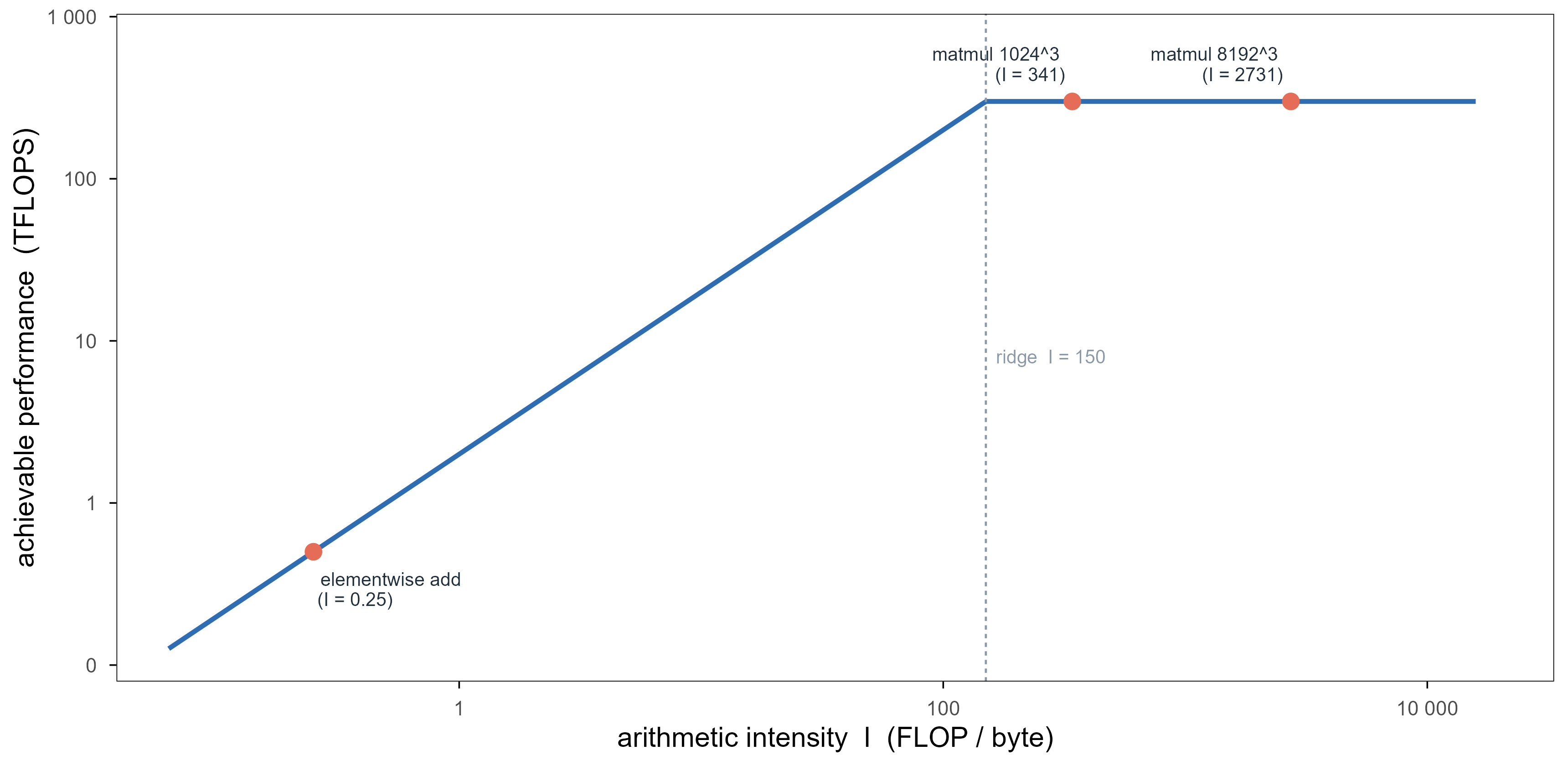
Larger \(I\) is better value; smaller \(I\) means the program is moving data rather than computing. Two real numbers show the spread: a \(1024^3\) fp16 matmul does \(2\times1024^3=2.15\times10^{9}\) FLOPs while moving \(3\times1024^2\times2=6.29\) MB, so \(I\approx341\); an elementwise add does one FLOP per element and moves 2 bytes in plus 2 out, so \(I=0.25\). That is a factor of 1360.
Figure 14: Roofline 模型。斜线段受带宽限制(\(\text{性能}=\text{带宽}\times I\)),水平段受峰值算力限制。设峰值 300 TFLOPS、带宽 2000 GB/s,转折点在 \(I=150\)。逐元素加法落在斜线上(受带宽限制),两个矩阵乘落在水平段(受算力限制)。 | The roofline model. The sloped part is bandwidth-limited (\(\text{perf}=\text{bandwidth}\times I\)); the flat part is compute-limited. With a 300 TFLOPS peak and 2000 GB/s of bandwidth the ridge sits at \(I=150\). An elementwise add lands on the slope (bandwidth-bound); both matmuls land on the plateau (compute-bound).
This figure explains why “optimising an operator” usually means “moving fewer bytes”: if the operator sits on the slope, doubling peak compute changes nothing — bandwidth is the ceiling.
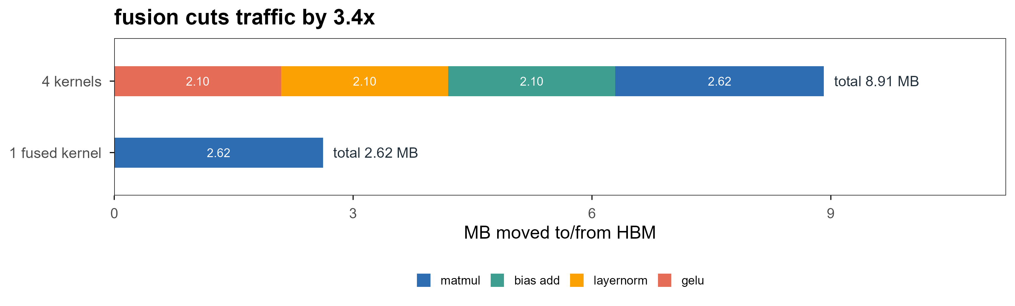
Operator fusion is the most basic lever. A LayerNorm → GELU sequence naively launches two kernels, each writing a full tensor back to memory and reading it again; once fused there is one read and one write.
Figure 15: 算子融合前后的显存往返。设 fp16、\(N=1024\)、\(d=512\):激活张量 1.05 MB,权重 0.52 MB。四个独立 kernel 一共搬 8.91 MB,融合成一个 kernel 后只需 2.62 MB,约为原来的 1/3.4。这是按张量形状算出的下界,不是实测时间。 | Memory traffic before and after fusion. With fp16, \(N=1024\), \(d=512\): a 1.05 MB activation and a 0.52 MB weight. Four separate kernels move 8.91 MB; a single fused kernel needs 2.62 MB, about 1/3.4. This is a lower bound computed from tensor shapes, not a measured runtime.
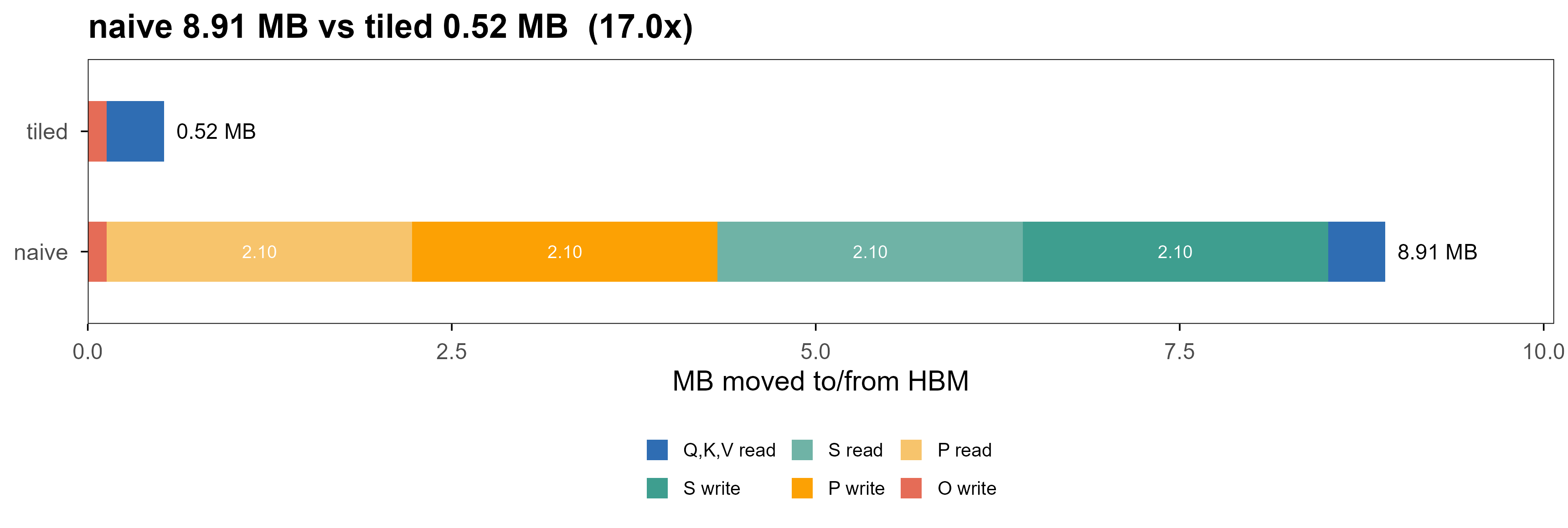
FlashAttention is the same logic taken to the limit. Section 3.6 decomposed attention into four boxes; the naive implementation writes the full \(n\times n\) score matrix to memory. At \(n=1024\), \(d=64\), fp16, that matrix is 2.10 MB while \(Q,K,V\) are 0.13 MB each. The score matrix is written once and read once, then the same again after softmax — the \(n^2\) round trips completely dominate the actual arithmetic.
Code
N <-1024; d <-64; bpp <-2sz_nd <- N * d * bpp /1e6# MB per N x d tensorsz_nn <- N * N * bpp /1e6# MB per N x N matrixflash <-data.frame(item =c("Q,K,V read", "S write", "S read", "P write", "P read", "O write"),mb =c(3* sz_nd, sz_nn, sz_nn, sz_nn, sz_nn, sz_nd),path ="naive")f2 <-data.frame(item =c("Q,K,V read", "O write"),mb =c(3* sz_nd, sz_nd), path ="tiled")fl <-rbind(flash, f2)fl$item <-factor(fl$item, levels =c("Q,K,V read", "S write", "S read","P write", "P read", "O write"))fl$path <-factor(fl$path, levels =c("naive", "tiled"))tot2 <-data.frame(path =factor(c("naive", "tiled"), levels =c("naive", "tiled")),mb =c(sum(flash$mb), sum(f2$mb)))ggplot(fl, aes(mb, path, fill = item)) +geom_col(width =0.5) +geom_text(aes(label =ifelse(mb >0.4, sprintf("%.2f", mb), "")),position =position_stack(vjust =0.5), size =2.5, colour ="white") +geom_text(data = tot2, aes(mb, path, label =sprintf("%.2f MB", mb)),inherit.aes =FALSE, hjust =-0.15, size =3) +scale_fill_manual(values =c("Q,K,V read"= op_pal[["blue"]], "S write"= op_pal[["teal"]],"S read"="#6FB3A6", "P write"= op_pal[["orange"]],"P read"="#F7C46C", "O write"= op_pal[["coral"]]),name =NULL) +scale_x_continuous(expand =expansion(mult =c(0, 0.13))) +labs(x ="MB moved to/from HBM", y =NULL,title =sprintf("naive %.2f MB vs tiled %.2f MB (%.1fx)",sum(flash$mb), sum(f2$mb), sum(flash$mb) /sum(f2$mb))) +theme(axis.text.y =element_text(size =9), legend.text =element_text(size =7.4),legend.key.size =unit(0.34, "cm"), legend.position ="bottom")
Figure 16: 注意力在 \(N=1024\)、\(d=64\)、fp16 下的 HBM 往返(MB)。朴素实现把 \(N\times N\) 的分数矩阵与概率矩阵物化,四次往返共 8.91 MB;分块实现让 \(N\times N\) 块留在片上 SRAM,只搬 \(Q,K,V\) 与输出,共 0.52 MB,相差约 17 倍。 | HBM traffic for attention at \(N=1024\), \(d=64\), fp16, in MB. The naive path materialises the \(N\times N\) score and probability matrices: four round trips, 8.91 MB. The tiled path keeps \(N\times N\) tiles in on-chip SRAM and only moves \(Q,K,V\) plus the output: 0.52 MB, roughly 17x less.
The crucial point: FlashAttention does not change the mathematics of attention. It tiles \(Q,K,V\) into on-chip memory, accumulates with an online softmax, and recomputes intermediates in the backward pass instead of storing them. The output is numerically equivalent to the standard path (differences at the level of floating-point error), so it belongs to the second kind, not the first. The authors report 2–4x single-operator speedups, varying with sequence length, head dimension and hardware; what is worth remembering is the judgement: it saves bytes, not FLOPs — FLOPs even rise slightly because of recomputation.
The criterion for the second kind is therefore blunt: is the output equivalent? If so, it may only be compared on time, memory and energy — never advertised as “better results”.
5.4 第三类:换整体设计 / Third kind: change the design
第三类连算子都不换,换的是拼装方式:
The third kind does not even change the operators; it changes how they are wired:
残差连接:\(y=x+f(x)\)。\(f\) 里的算子一个没变,但梯度多了一条恒等通路,深层网络才训得动。 Residual connections: \(y=x+f(x)\). Not one operator inside \(f\) changes, yet gradients get an identity path and deep networks become trainable.
归一化的位置:pre-LN 与 post-LN 用的是同一个 LayerNorm,训练稳定性差别很大。 Placement of normalisation: pre-LN and post-LN use the same LayerNorm, with very different training stability.
混合专家(MoE):把一个大前馈层换成若干专家加一个路由。路由是新的,专家内部的算子还是原来的。 Mixture of experts: one large feed-forward layer becomes several experts plus a router. The router is new; the operators inside each expert are the same.
KV 缓存:推理时把已经算过的键值存下来,不改变任何数学,只改变重复计算。 The KV cache: store keys and values already computed, changing no mathematics, only recomputation.
The value of such changes can far exceed that of any single operator, but they should not be described as “new operators”. The converse also holds: a mathematically elegant new operator that conflicts with its surroundings (say, it breaks a normalisation’s scale assumption) may deliver nothing end to end.
5.5 三类对照 / The three kinds side by side
第一类 机制 / mechanism
第二类 实现 / implementation
第三类 设计 / design
改变了什么 / changes
数学映射本身 / the mapping itself
数据怎么搬 / how data moves
算子怎么拼 / how ops are wired
输出是否等价 / output equivalent
不等价 / no
等价 / yes
不等价 / no
该用什么指标 / metric
表达能力、同预算下的精度、泛化 / expressiveness, accuracy at equal budget, generalisation
延迟、吞吐、显存峰值、能耗 / latency, throughput, peak memory, energy
端到端指标、训练稳定性、数据效率 / end-to-end metrics, stability, data efficiency
典型例子 / examples
GIN 的求和聚合、GAT、RGAT / sum aggregation in GIN, GAT, RGAT
With this table the question list at the end of section 8 has a basis. First, a more fundamental question: if you really want to build a new operator, where do you start?
6. 能不能自己发明一种算子? / Can you invent an operator yourself?
Yes, and the barrier is lower than it looks. What is hard is not writing the formula but showing it deserves to exist. Start from the plainest linear expression and add one thing at a time, watching what each step buys and what it costs.
6.1 一步步把一个线性式改造掉 / Mutating a linear expression, one step at a time
第 0 步:\(y=wx\)。一个标量权重,能表达的只有过原点的直线。
Step 0: \(y=wx\). One scalar weight; the only functions it can express are lines through the origin.
第 1 步:\(y=wx+b\)。加一个偏置,直线可以平移。参数量 1 → 2,能力没有质变。
Step 1: \(y=wx+b\). Add a bias and the line can shift. Parameters go 1 → 2; nothing qualitative changes.
Step 2: \(y=\sigma(wx+b)\). Wrap it in a nonlinearity. This is where things change qualitatively: a single perceptron still cannot represent XOR, but a few of these units side by side, stacked one more layer, can represent any continuous function (universal approximation). Note that “can represent” is not “can represent with few parameters” — that gap is the root of every later argument.
Step 3: \(y=w_1x_1+w_2x_2+w_{12}x_1x_2\). Add an interaction term. In the first two steps the two inputs contribute separately and are then summed; with \(x_1x_2\) the effect of one input depends on the value of the other. In statistical language this moves from a main-effects model to one with interactions.
Step 4: \(y_i=\sum_j a_{ij}(x)\,v_j\), where \(a_{ij}\) is a function of the input and \(\sum_j a_{ij}=1\). That is the skeleton of attention. Compare it with step 0 and the mathematical form is almost identical: the only difference is that the weights are no longer parameters but functions of the input. That single change is why attention is powerful, and also why it is expensive — the weights must be recomputed for every new input.
Step 5: \(y_i=\sum_{r}\sum_{j\in\mathcal{N}_r(i)} a_{ij}^{(r)}(x)\,W_r\,v_j\). Add adjacency and relation types and you have the RGAT of section 4. By now “operator” spans the whole range from 2 parameters to hundreds of millions.
What is worth remembering is that each step changed exactly one thing. Almost every new operator that gets cited can be decomposed this way — some component of some step was swapped — rather than appearing out of nowhere.
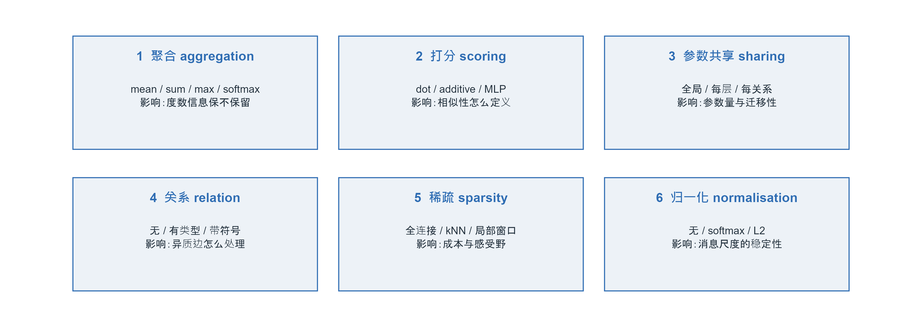
6.2 六个可以拧的旋钮 / Six knobs you can turn
把 3.7 节那个消息传递公式拆开,可调的地方其实不多:
Decompose the message-passing formula from section 3.7 and there are only a few places to intervene:
Figure 17: 设计一个新算子时可以拧的六个旋钮。每个旋钮下面给出可选做法与它主要影响的东西。真正的新算子通常只动其中一两个,其余保持不变——这也是做消融实验时该控制的变量。 | Six knobs available when designing an operator, each with its options and what it mainly affects. A genuine new operator usually turns only one or two of them and leaves the rest fixed — which is exactly what an ablation must control for.
An honest caveat: the six knobs are not independent. Changing the aggregation changes gradient scale, changing sparsity changes the effective receptive field, changing normalisation changes the optimal learning rate. So an experiment that “swaps one operator” usually needs its hyperparameters retuned before the comparison is fair — and that missing step explains many “the new operator is better” claims.
6.3 一个能跑的小实验:聚合函数不是中立的 / A runnable experiment: aggregation is not neutral
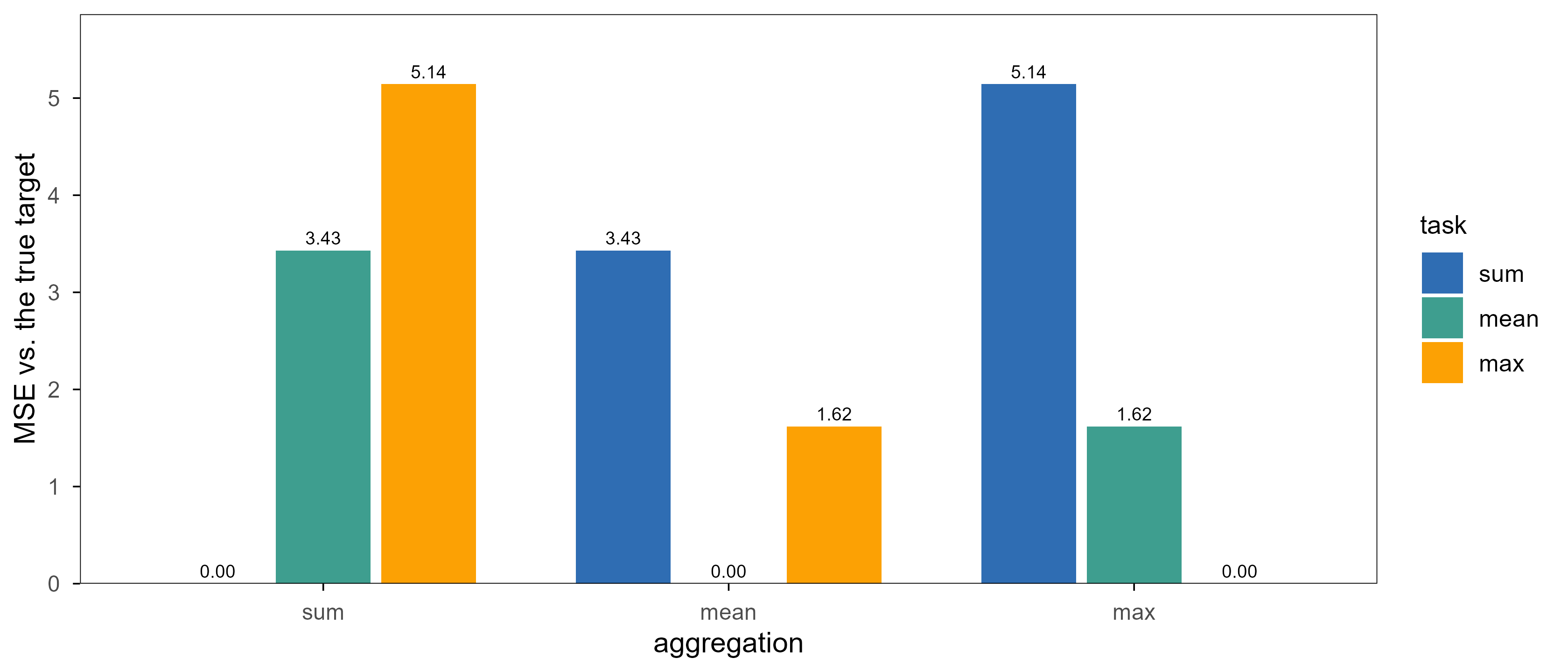
Take 400 synthetic nodes with 5 neighbours each, neighbour values drawn from a standard normal. Define three tasks — predict the sum, the mean and the max of the neighbours — then fit each with each of the three aggregations and compare mean squared error.
Code
set.seed(20261029)G <-400; K <-5H <-matrix(rnorm(G * K), G, K)truth <-list(sum =rowSums(H), mean =rowMeans(H), max =apply(H, 1, max))fitted <-list(sum =rowSums(H), mean =rowMeans(H), max =apply(H, 1, max))grid <-expand.grid(agg =names(fitted), task =names(truth), stringsAsFactors =FALSE)grid$mse <-mapply(function(a, t) mean((fitted[[a]] - truth[[t]])^2), grid$agg, grid$task)grid$agg <-factor(grid$agg, levels =c("sum", "mean", "max"))grid$task <-factor(grid$task, levels =c("sum", "mean", "max"))ggplot(grid, aes(agg, mse, fill = task)) +geom_col(position =position_dodge(width =0.78), width =0.7) +geom_text(aes(label =sprintf("%.2f", mse)),position =position_dodge(width =0.78), vjust =-0.45, size =2.5) +scale_fill_manual(values =unname(op_pal[c("blue", "teal", "orange")]),name ="task") +scale_y_continuous(expand =expansion(mult =c(0, 0.14))) +labs(x ="aggregation", y ="MSE vs. the true target") +theme(legend.position ="right")
Figure 18: 聚合函数与任务假设必须匹配。固定读出(直接用聚合值作预测)时,对角线上误差为 0,非对角线落在 1.6–5.1 之间。注意这只说明「聚合编码了假设」,不说明某种聚合普遍更差——若下游有可学习的读出层,知道度数时求和可以精确还原均值。 | Aggregation must match the task assumption. With a fixed readout (the aggregate is the prediction), the diagonal has zero error and off-diagonal entries lie between 1.6 and 5.1. This shows that aggregation encodes an assumption; it does not show that any aggregation is universally worse — with a learnable readout and known degree, a sum reconstructs the mean exactly.
Read it directly: in each row exactly one bar has height zero. There is no universally best aggregation, only one that matches the task assumption. This reconciles two apparently contradictory facts: GIN proves that sum is the most expressive aggregation (it distinguishes multisets, whereas the mean erases the degree), yet in this experiment the mean has zero error on its own task. Both are right — expressiveness is about what can be represented; error is about how well it is represented on this task.
6.4 什么才算有意义的创新 / What counts as a meaningful contribution
把上面的讨论收成一份清单。一个新的算子要成立,至少得在下面几项里站住一项,并且在其余项上不塌:
Condense the discussion into a checklist. For a new operator to stand, it must win on at least one of these and not collapse on the others:
新的数学运算或参数化:确实定义了一个之前没有的映射,而不仅是重命名。 A genuinely new operation or parameterisation: a mapping that did not exist before, not a renaming.
不同的归纳偏置:假设改变了,而且这个新假设与目标任务的结构相符。 A different inductive bias: the assumption changed, and the new assumption matches the structure of the target task.
更合理的信息传播:多跳、异质、带符号、带方向的信息如何汇合,有了明确的机制而不是靠加深层数硬凑。 More sensible information propagation: a mechanism for multi-hop, heterogeneous, signed or directed information instead of brute-force depth.
更高的计算效率:单位效果的成本下降,且这种下降来自结构而不是实现技巧。 Higher efficiency: lower cost per unit of performance, and the gain comes from structure rather than implementation tricks.
更好的预测性能:在同参数、同数据、同预算下比较,并且报告方差与训练成本。 Better predictive performance: compared at equal parameters, data and budget, with variance and training cost reported.
更可靠的泛化:跨数据集、跨规模(序列更长、图更大、物种不同)仍然成立。 More reliable generalisation: it survives across datasets and across scale — longer sequences, larger graphs, different species.
The order of validation matters; getting it wrong produces false positives. Start with theory (expressiveness, equivariance, complexity), then a controlled ablation (one change at a time, each with its own tuned hyperparameters), and only then a benchmark (several tasks, several seeds, mean and standard deviation). Skip to the last step alone and you will almost always find some dataset where the numbers look better.
One more thing is routinely omitted: report the negative results. Stating the conditions under which an operator is worse is more valuable than hiding them — it tells the next person exactly where the boundary lies.
7. AI 虚拟细胞需要什么样的算子? / What operators does a virtual cell need?
Most examples so far came from images and language. Biology differs: the data are sparser and noisier, interventions are expensive, and causality lives in the structure. This section puts operators back into a biological setting.
7.1 生物学问题长什么样 / What the biological problem looks like
Take Perturb-seq: knock out a gene with CRISPR, then read the transcriptome of thousands of single cells. The result is paired data of “perturbation → expression change”. The usual goal is to predict perturbations that were never performed, not to memorise the ones that were.
这件事难在三点,每一点都直接指向算子的选择:
Three things make it hard, and each points straight at a choice of operator:
稀疏且高维:一个细胞里多数基因的计数是 0,信噪比很低。归一化和聚合方式会显著影响结果。 Sparse and high-dimensional: most genes in a cell have zero counts and the signal-to-noise ratio is low. Normalisation and aggregation matter a lot.
结构先验是已知的:基因不是独立变量,调控关系、通路成员、蛋白互作都是已知知识。用不用、怎么用,是归纳偏置的问题。 Structural priors exist: genes are not independent; regulatory relations, pathway membership and protein interactions are known. Whether and how to use them is a question of inductive bias.
干预有方向、有符号:激活和抑制是两件事,敲除和过表达也是两件事。把它们压成同一种边,会丢掉关键信息。 Interventions have direction and sign: activation and inhibition differ, and so do knockout and overexpression. Collapsing them into one kind of edge discards the key information.
7.2 一个 5 个基因的调控网络 / A five-gene regulatory network
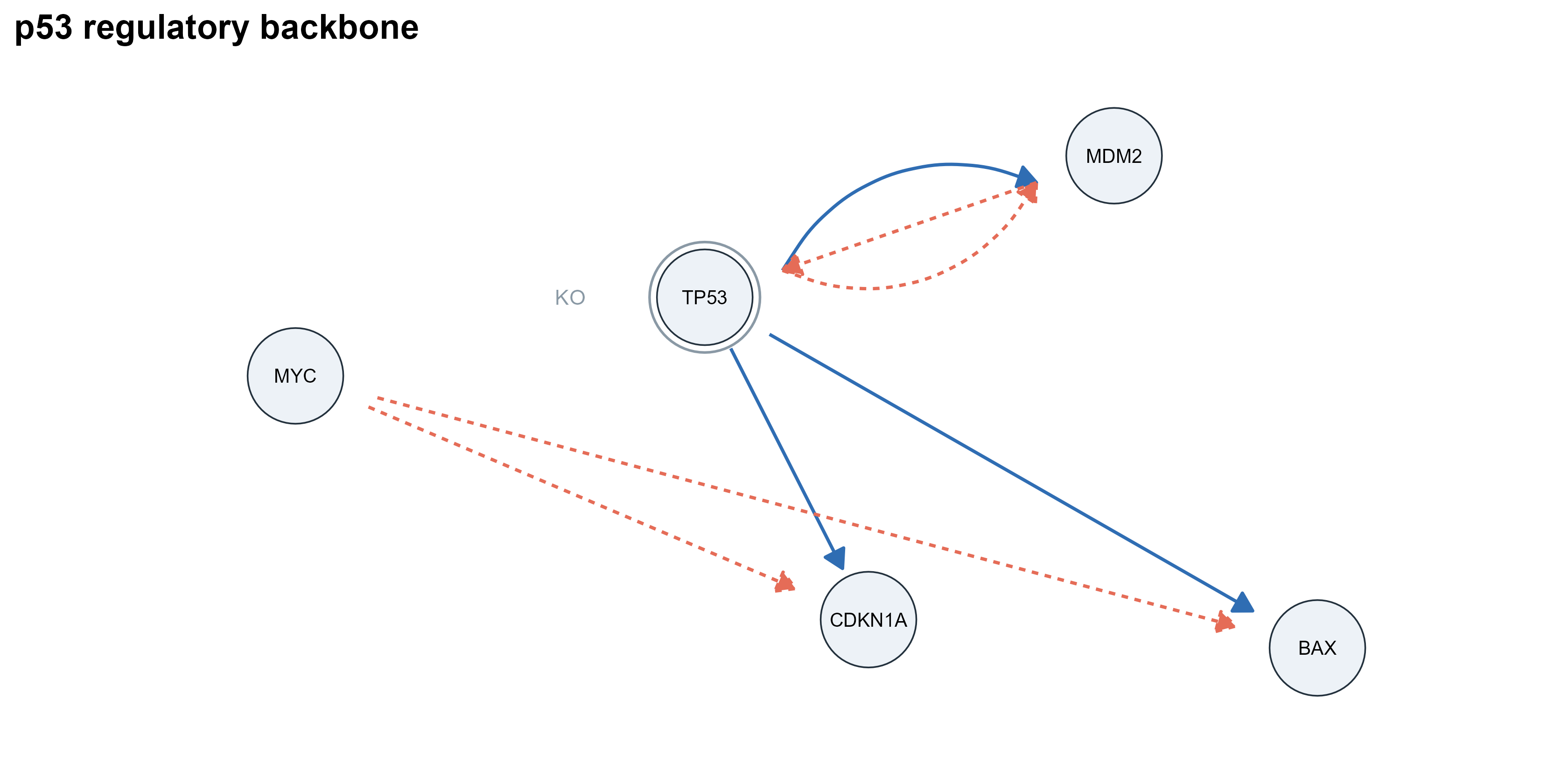
The network below is the textbook p53 backbone, trimmed to five genes and six edges. The signs are not decoration: TP53 transcriptionally activates MDM2, MDM2 inhibits TP53 in return (negative feedback), TP53 activates CDKN1A and BAX, and MYC inhibits CDKN1A and BAX.
Figure 19: 一个 5 基因的调控网络。实线蓝箭头表示激活(TP53→MDM2、TP53→CDKN1A、TP53→BAX),虚线珊瑚线表示抑制(MDM2⊣TP53、MYC⊣CDKN1A、MYC⊣BAX)。TP53 与 MDM2 构成负反馈环,这是整张网络里最需要「关系感知」的一处:任何把它们当成对称边的模型都会算错稳态。灰色圈标出下文被扰动的基因。 | A five-gene regulatory network. Solid blue arrows are activations (TP53→MDM2, TP53→CDKN1A, TP53→BAX) and dashed coral lines are inhibitions (MDM2⊣TP53, MYC⊣CDKN1A, MYC⊣BAX). TP53 and MDM2 form a negative-feedback loop — the place where relation-awareness matters most: any model that treats them as symmetric edges gets the steady state wrong. The grey ring marks the gene perturbed below.
Every sign here enters the computation. Take the absolute value of \(-0.7\) and “MYC inhibits CDKN1A” becomes “MYC activates CDKN1A”, which flips the predicted direction of MYC overexpression entirely — section 7.3 works that example through.
7.3 扰动如何传播:符号在哪一步显形 / How a perturbation propagates, and where the sign shows up
Use a minimal linear dynamical model for cell state. At each step the expression vector \(h_t\) is driven by two things: its own decay and regulation from upstream genes.
The \((i,j)\) entry of \(W\) is the signed strength with which \(j\) regulates \(i\); \(b\) is basal transcription and \(\alpha\) sets the update rate. The steady state satisfies \(h^\ast=(I-W)^{-1}b\). A knockout clamps that component to 0 at every step, and overexpression clamps it higher — both are external constraints on one coordinate, with \(W\) untouched. This model is plainer than the \(\tanh\) version, which is exactly why it exposes what the sign does.
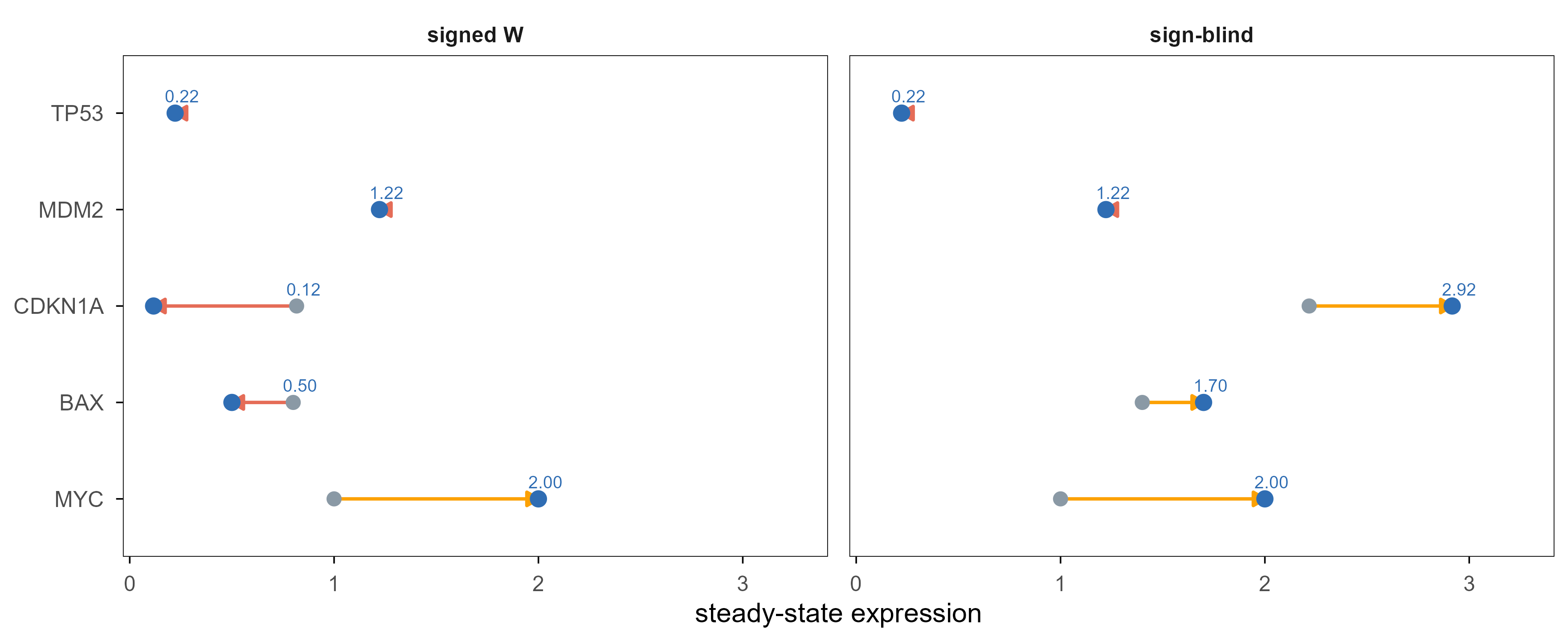
The experiment below clamps MYC at 2.0 (overexpression) and runs it in two models: one with the signed \(W\), and one where the two inhibitory edges have lost their sign.
Figure 20: MYC 过表达的稳态预测。每个面板是一个模型:实心点是基线,箭头指向过表达后的稳态。带符号的模型预测 CDKN1A 与 BAX 下降;把两条抑制边的符号去掉之后,同样的网络预测它们上升。TP53 与 MDM2 在两个面板里都不动,因为从 MYC 出发没有到达它们的路径。 | Predicted steady state under MYC overexpression. Each panel is one model: the solid dot is baseline and the arrow points to the overexpressed steady state. With signs, CDKN1A and BAX fall; after dropping the sign on the two inhibitory edges the same network predicts they rise. TP53 and MDM2 do not move in either panel, because no path from MYC reaches them.
Reading it: the signed model gives CDKN1A \(0.82\to0.12\) and BAX \(0.80\to0.50\), both falling; the sign-blind model gives \(2.22\to2.92\) and \(1.40\to1.70\), both rising. Same numbers, same graph, opposite directions — the only difference is whether “inhibition” had a place in the parameters.
One counter-intuitive detail deserves its own paragraph: switch the perturbation to a TP53 knockout and both models give identical changes (CDKN1A \(-0.27\), BAX \(-0.20\) in both). In a linear model the untouched MYC term cancels in the difference, so the sign error is completely hidden. In other words, a sign error only becomes visible when you perturb the very gene whose sign you got wrong. That is exactly why a benchmark built on a handful of perturbations easily misses structural errors: the perturbations you happened to test may sit where the error does not show.
That is the reason relation-aware operators exist. They are not a fancier scoring function but the only way for “inhibition” to occupy a place in the computation — and their value must be demonstrated on the right perturbation experiments, or a sign-blind model will tie with them on your benchmark.
7.4 非配对多组学:对齐是一个模块,不是一个算子 / Unpaired multi-omics: alignment is a module
Real data often lack paired samples: one batch of cells has RNA, another has ATAC, from different patients and batches. Comparing them in one space requires alignment.
The usual approach learns a shared embedding: an encoder per modality maps cells into one space, and a contrastive loss pulls together samples that should represent the same state while pushing the rest apart. Other work solves for an explicit cross-modality matching with optimal transport.
By the taxonomy of section 5, most of this work is module level: a contrastive loss is a training objective, not an operator in the forward pass; an optimal-transport solver is a step in the training loop and never enters the inference graph. The value can be enormous, but calling it a “new operator” hides the mechanism actually at work — what enters inference is still the linear layers, attention and normalisation inside the encoders.
7.5 先验该有多硬 / How hard should the prior be
同一个生物学网络,可以用三种强度塞进模型:
The same biological network can be injected at three strengths:
硬先验:把调控边写死成邻接矩阵,模型只能在这些边上传递消息。省数据、可解释,但发现不了新机制——没被写进网络的调控关系永远不会被预测出来。 Hard prior: bake the edges into the adjacency matrix; messages may only travel along them. Data-efficient and interpretable, but unable to discover new mechanisms — a regulation absent from the network can never be predicted.
软先验:把已知边作为初始权重或额外的注意力偏置,允许模型偏离。既能利用知识,又保留余地。 Soft prior: use known edges as initial weights or as an additive bias on attention, letting the model deviate. It exploits knowledge while leaving room.
学出来的结构:从数据里推断图(例如用基因共表达或注意力权重反推),先验只体现在”稀疏”“低秩”这类约束上。数据需求大,但可能发现未记录的调控。 Learned structure: infer the graph from data (say, from co-expression or attention weights), with the prior living only in constraints such as sparsity or low rank. Data-hungry, but able to surface undocumented regulation.
None of the three is right or wrong; only the match to the question matters. For predicting a knockout inside a known pathway, a hard prior is usually the best value; for finding new regulators it is self-imposed blindness. Existing virtual-cell models sit at different points: GEARS uses gene-ontology graphs as an inductive bias for perturbation prediction, while scGPT and Geneformer pretrain on large single-cell corpora and fine-tune on smaller perturbation sets. Their difference is not “whose operator is more advanced” but how much biological structure is written into the computation.
8. 总结:算子、架构与能力 / Operators, architectures and capability
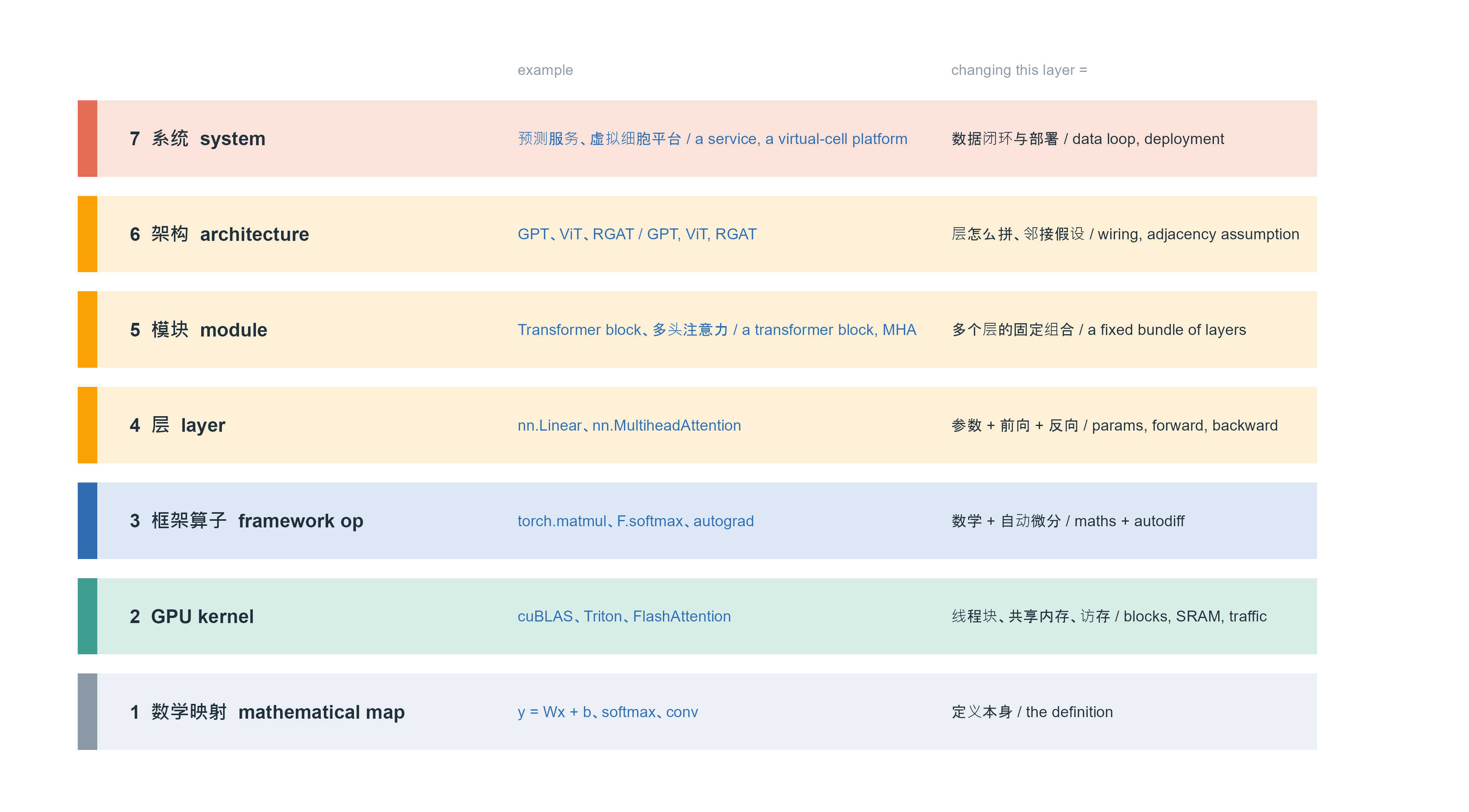
Eight sections have split the word “operator” into several layers. One figure stacks them back together, bottom to top: the lower you go, the more abstract and definitional; the higher, the more concrete and product-like.
Code
hier <-data.frame(y =7:1,name =c("7 系统 system", "6 架构 architecture", "5 模块 module","4 层 layer", "3 框架算子 framework op", "2 GPU kernel","1 数学映射 mathematical map"),ex =c("预测服务、虚拟细胞平台 / a service, a virtual-cell platform","GPT、ViT、RGAT / GPT, ViT, RGAT","Transformer block、多头注意力 / a transformer block, MHA","nn.Linear、nn.MultiheadAttention","torch.matmul、F.softmax、autograd","cuBLAS、Triton、FlashAttention","y = Wx + b、softmax、conv"),mean =c("数据闭环与部署 / data loop, deployment","层怎么拼、邻接假设 / wiring, adjacency assumption","多个层的固定组合 / a fixed bundle of layers","参数 + 前向 + 反向 / params, forward, backward","数学 + 自动微分 / maths + autodiff","线程块、共享内存、访存 / blocks, SRAM, traffic","定义本身 / the definition"),grp =c("sys", "arch", "arch", "arch", "fw", "ker", "math"))hier$fill <-c(sys ="#FBE3D9", arch ="#FDF0D8", fw ="#DCE8F5",ker ="#D8EDE7", math ="#EAF0F5")[hier$grp]hier$bar <-c(sys = op_pal[["coral"]], arch = op_pal[["orange"]], fw = op_pal[["blue"]],ker = op_pal[["teal"]], math = op_pal[["grey"]])[hier$grp]ggplot(hier) +geom_rect(aes(xmin =0, xmax =10, ymin = y -0.4, ymax = y +0.4), fill = hier$fill) +geom_rect(aes(xmin =0, xmax =0.16, ymin = y -0.4, ymax = y +0.4),fill = hier$bar, colour =NA) +geom_text(aes(0.42, y, label = name), hjust =0, size =3.1, fontface ="bold",colour = op_pal[["ink"]]) +geom_text(aes(3.55, y, label = ex), hjust =0, size =2.5,colour = op_pal[["blue"]]) +geom_text(aes(7.05, y, label = mean), hjust =0, size =2.5,colour = op_pal[["ink"]]) +annotate("text", x =3.55, y =7.72, label ="example", size =2.4,colour = op_pal[["grey"]], hjust =0) +annotate("text", x =7.05, y =7.72, label ="changing this layer =", size =2.4,colour = op_pal[["grey"]], hjust =0) +coord_cartesian(xlim =c(0, 10.6), ylim =c(0.45, 7.95)) + plain
Figure 21: 算子的七层结构。第 1–2 层回答「做什么」,第 3 层回答「怎么在芯片上做」,第 4–6 层回答「怎么搭」,第 7 层是最终交付的系统。每往上一层,可替换的部件变多、单次改动的影响变大,但都不改变下层已经确定的数学。 | Seven layers. Layers 1–2 answer 「what is done」, layer 3 answers 「how it is done on silicon」, layers 4–6 answer 「how it is assembled」, and layer 7 is the delivered system. Going up, more parts become swappable and a single change has wider impact — but none of it changes the mathematics already fixed below.
这张图最实用的地方,是把它当成”定位器”用。听到一句关于算子的话,先问它落在第几层:
The most practical use of this figure is as a locator. When you hear a claim about an operator, first ask which layer it lives on:
“我们提出了新的注意力机制” → 第 1–2 层(换数学)。 “We propose a new attention mechanism” → layers 1–2 (new mathematics).
“我们把注意力的显存降了 10 倍” → 第 3 层(换 kernel,数学不变)。 “We cut attention’s memory 10x” → layer 3 (new kernel, same mathematics).
“我们把 LayerNorm 移到注意力之前” → 第 4–6 层(换拼装)。 “We moved LayerNorm before attention” → layers 4–6 (new wiring).
“我们的模型在细胞扰动预测上更强” → 第 7 层(系统级结果),需要回头找原因。 “Our model predicts perturbations better” → layer 7 (a system-level result) that needs its cause traced back down.
The relationship compresses into one sentence: operators fix which functions can be expressed and at what cost; architectures fix how those functions are composed to match the structure of the data; capability is the joint outcome of both plus data and scale, never something a single operator supplies on its own.
8.1 听到”更好的算子”时该问什么 / Questions to ask about a “better operator”
把全篇的判据收成八问。前四问用来定位,后四问用来验证:
Collect the criteria into eight questions. The first four locate the claim; the last four test it:
它改的是哪一层?能不能给出改动前后两个公式?如果给不出,多半是第 3 层或第 6 层。 Which layer does it change? Can it show the formula before and after? If not, it is probably layer 3 or layer 6.
输出与谁等价?若与标准实现数值等价,就不能用”效果更好”作为卖点,只能比时间、显存、能耗。 What is its output equivalent to? If numerically equal to a standard implementation, “better results” is not a selling point; only time, memory and energy are.
参数量、FLOPs、显存、算术强度各是多少?落在 roofline 的斜线一侧还是水平段? What are the parameter count, FLOPs, memory and arithmetic intensity? Which side of the roofline?
它假设了什么结构?这个假设在你的数据上成立吗?反过来,在什么数据上必然失效? What structure does it assume? Does that hold for your data — and on what data must it fail?
消融是否只改了这一处?新旧两版的超参数是否各自调过?随机种子有几个,方差多大? Does the ablation change only this one thing? Were both versions tuned separately? How many seeds, and what is the variance?
是否同参数、同数据、同训练预算?把一个算子塞进三倍大的模型里比较,得到的不是算子的功劳。 Equal parameters, data and training budget? Putting an operator inside a 3x larger model is not evidence for the operator.
规模变了还成立吗?序列更长、图更大、物种不同、批次不同,结论是否保持? Does it survive scale — longer sequences, larger graphs, different species, different batches?
负结果在哪里?作者有没有说清楚它在什么条件下更差?一条都没有的论文,通常不是因为它处处更好。 Where are the negative results? Does the paper say when it is worse? A paper with none usually is not better everywhere.
These eight questions need no code to ask, yet they turn most marketing into testable statements. Back to \(2\times3=6\) from the opening: from that line to today’s virtual cells, the thread is the same — write down clearly how inputs become outputs, and say honestly where that writing holds.
参考文献 / References
Vaswani, A., et al. (2017). Attention is all you need. NeurIPS. arXiv:1706.03762
Kipf, T. N. & Welling, M. (2017). Semi-supervised classification with graph convolutional networks. ICLR. arXiv:1609.02907
Veličković, P., et al. (2018). Graph attention networks. ICLR. arXiv:1710.10903
Xu, K., et al. (2019). How powerful are graph neural networks? ICLR. arXiv:1810.00826
Gilmer, J., et al. (2017). Neural message passing for quantum chemistry. ICML. arXiv:1704.01212
Schlichtkrull, M., et al. (2018). Modeling relational data with graph convolutional networks. ESWC. arXiv:1703.06103
Busbridge, D., et al. (2019). Relational graph attention networks. arXiv:1904.05811
Dao, T., et al. (2022). FlashAttention: fast and memory-efficient exact attention with IO-awareness. NeurIPS. arXiv:2205.14135
Katharopoulos, A., et al. (2020). Transformers are RNNs: fast autoregressive transformers with linear attention. ICML. arXiv:2006.16236
Assran, M., et al. (2023). Self-supervised learning from images with a joint-embedding predictive architecture. CVPR. arXiv:2301.08243
He, K., et al. (2016). Deep residual learning for image recognition. CVPR. arXiv:1512.03385
Shazeer, N., et al. (2017). Outrageously large neural networks: the sparsely-gated mixture-of-experts layer. ICLR. arXiv:1701.06538
Chen, T., et al. (2018). TVM: an automated end-to-end optimizing compiler for deep learning. OSDI. arXiv:1802.04799
Williams, S., Waterman, A. & Patterson, D. (2009). Roofline: an insightful visual performance model for multicore architectures. Communications of the ACM 52(4), 65–76.
Theodoris, C. V., et al. (2023). Transfer learning enables predictions in network biology. Nature 618, 616–624. doi:10.1038/s41586-023-06139-9
Cui, H., et al. (2024). scGPT: toward building a foundation model for single-cell multi-omics using generative AI. Nature Methods 21, 1470–1480.
Roohani, Y., et al. (2024). Predicting transcriptional outcomes of novel multigene perturbations with GEARS. Nature Biotechnology 42, 927–936. arXiv:2304.12783
Replogle, J. M., et al. (2022). Mapping information-rich genotype–phenotype landscapes with genome-scale Perturb-seq. Cell 185(14), 2559–2575.
PyTorch documentation. torch.matmul, torch.nn.functional, and the ATen operator registry. https://pytorch.org/docs/stable/
Dosovitskiy, A., et al. (2021). An image is worth 16x16 words: transformers for image recognition at scale. ICLR. arXiv:2010.11929
Isensee, F., et al. (2021). nnU-Net: a self-configuring method for deep learning-based biomedical image segmentation. Nature Methods 18, 203–211.
Avsec, Ž., et al. (2021). Effective gene expression prediction from sequence by integrating long-range interactions. Nature Methods 18, 1196–1203.
Lin, Z., et al. (2023). Evolutionary-scale prediction of atomic-level protein structure with a language model. Science 379, 1123–1130.
Himmelstein, D. S., et al. (2017). Systematic integration of biomedical knowledge prioritizes drugs for repurposing. eLife 6, e26726.
Citation note: entries 1–13, 17 and 20 give arXiv identifiers; check the journal record for the version of record. Entries 14–16, 18 and 21–24 give volume and pages; verify against the journal before citing where no DOI is given. Entry 19 is official documentation.