This post was drafted by an AI system (DeepSeek-Flash). Every number in it comes from actually running the code below on the author’s machine, but the prose has not been proofread line by line. Paths to Python and R are absolute paths on that machine and must be adapted elsewhere.
1. 这个测试想回答什么 / What this test tries to answer
这篇不是教程,更像一次环境审计。我把三件事塞进了同一份 .qmd:两边各自训练一个小模型、比较两边的数值、检查 Quarto 的多种 chunk 引擎到底哪几个会在渲染时真正执行。
This is less a tutorial than an environment audit. I put three things into a single .qmd: train a small model in each framework, compare the two numerically, and check which of Quarto’s chunk engines actually execute during rendering.
具体来说有三个问题:
两个框架能不能在同一台机器上同时跑通? R 的 torch 包和 Python 的 PyTorch 都封装了 libtorch,但它们的 Windows 二进制分发是两条独立的路径,坑也不一样。
Quarto 的 chunk 引擎是不是”什么语言都能写”? 文档里能写 {julia} 不代表渲染时它会执行;有些引擎只是把代码原样搬到 HTML 里。
Three questions, more precisely:
Can both frameworks run on the same machine? R’s torch package and Python’s PyTorch both wrap libtorch, but their Windows binaries ship along separate paths and fail in different ways.
On identical data and identical architecture, how different are convergence and runtime? “Both work” is not enough; I want to know whether they produce equivalent results.
Do Quarto chunk engines really mean “any language”? Being able to write a {julia} chunk does not mean it executes; some engines only ship the code to the browser.
Both frameworks run on CPU only. That matters: the timings below say something about overhead at this scale, and nothing about GPU training.
3. 哪些 chunk 引擎真的会执行 / Which chunk engines actually run
Quarto 允许在同一个文档里混用多种引擎,但”可写”和”可执行”是两件事。下表是本机的实测结果,后面的小节会逐个给出证据。
Quarto lets one document mix engines freely, but “can be written” and “can be executed” are different things. The table below is what this machine actually did; later sections show the evidence.
The {ojs} row is the one most often misread: OJS code does not run at render time at all. Quarto embeds a JavaScript module into the HTML and the page evaluates it when a reader opens it. “This code ran successfully” therefore can never be confirmed from the render log.
4. 同一个任务,两个框架 / One task, two frameworks
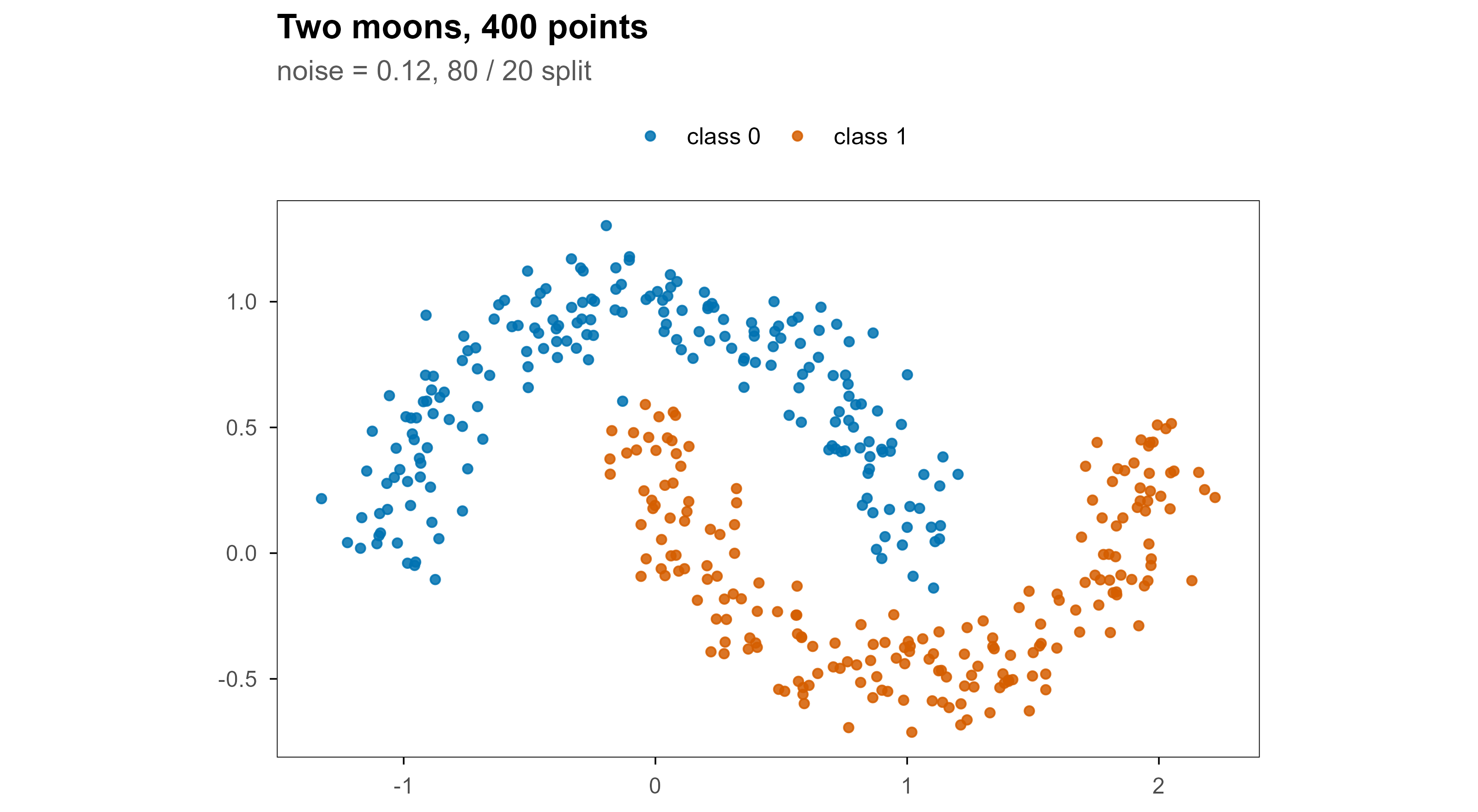
任务刻意选得很小:二维平面上的两个半月形(two moons),400 个点,320 个训练、80 个测试,两层 MLP(2 → 16 → 2),交叉熵损失,Adam,学习率 0.05,全批量训练 200 轮。这个规模小到 CPU 上几秒钟就能跑完,同时又足够让两个框架的 API 差异暴露出来。
The task is deliberately small: two interleaved half-moons in the plane, 400 points split into 320 train and 80 test, a two-layer MLP (2 → 16 → 2), cross-entropy loss, Adam with learning rate 0.05, full-batch training for 200 epochs. It is small enough to finish in seconds on a CPU, yet large enough to expose API differences between the frameworks.
数据只生成一次,由 Python 生成,然后写成一个 CSV 给 R 侧读。这样两边的差别只剩”框架”,而不是”数据”。
The data are generated once, in Python, then handed to R as a CSV. That leaves the framework as the only difference.
Code
import numpy as nprng = np.random.default_rng(7)def make_moons(n=400, noise=0.12): half = n //2 t = rng.uniform(0, np.pi, half) outer = np.c_[np.cos(t), np.sin(t)] inner = np.c_[1- np.cos(t), 0.5- np.sin(t)] X = np.r_[outer, inner] + rng.normal(0, noise, (n, 2)) y = np.r_[np.zeros(half), np.ones(half)].astype(int)return X.astype("float32"), yX, y = make_moons()# shared plotting / prediction grid: x varies fastest, y slowestgx = np.linspace(X[:, 0].min() -0.3, X[:, 0].max() +0.3, 80)gy = np.linspace(X[:, 1].min() -0.3, X[:, 1].max() +0.3, 80)# the R side runs in its own process, so the data travel through a CSVnp.savetxt(r.csv_path, np.c_[X, y], delimiter=",", header="x,y,label", comments="")print(f"X: {X.shape}, positives: {int(y.sum())} / {len(y)}")
The Python side is the textbook form: Sequential with two linear layers, CrossEntropyLoss, Adam. Loss is recorded every epoch, and the model then predicts on a grid to give a decision surface.
ver_py = torch.__version__check_py =float(torch.tensor([1.0, 2.0, 3.0]).exp().sum())print(f"torch {ver_py} | final loss {losses_py[-1]:.4f} | test acc {acc_py:.3f} | "f"load {t_load_py:.2f} s | train {t_train_py:.2f} s | infer {t_infer_py *1e3:.1f} ms")
torch 2.13.0+cpu | final loss 0.0050 | test acc 1.000 | load 1.77 s | train 0.15 s | infer 1.0 ms
6. 用 R 的 torch 训练 / Training with torch for R
R 侧的模型定义几乎是逐字对应:nn_sequential()、nn_linear()、nn_relu(),损失是 nnf_cross_entropy(),优化器是 optim_adam()。区别主要在两点:R 的标签张量必须是 1 起始的整数(torch_long()),以及所有方法都用 $ 调用而不是 .。
The R side maps almost one-to-one: nn_sequential(), nn_linear(), nn_relu(), loss as nnf_cross_entropy(), optimiser as optim_adam(). Two differences matter: R label tensors must be 1-based integers (torch_long()), and every method is called with $ instead of ..
The core of it is below (the full script is train-r-torch.R next to this post, kept in the repository rather than published with the page):
model <-nn_sequential(nn_linear(2, 16), nn_relu(), nn_linear(16, 2))opt <-optim_adam(model$parameters, lr =0.05)for (epoch inseq_len(200)) { opt$zero_grad() loss <-nnf_cross_entropy(model(Xtr), ytr) loss$backward() opt$step() losses[epoch] <-as.numeric(loss$item())}with_no_grad({ acc <-as.numeric( (model(Xte)$argmax(dim =2) == yte)$to(dtype =torch_float())$mean()$item() )})
注意这里有两个 R 特有的细节。第一,argmax(dim = 2) 里的 dim 是从 1 开始的,对应 Python 的 argmax(1)。第二,把张量转回 R 向量用 as.integer(),R 的 torch 张量没有 $numpy() 方法——第一次写的时候我照着 Python 的习惯写了 $cpu()$numpy(),得到的是一个和上下文毫无关系的报错(没有"fn"这个函数),而不是”方法不存在”。
Two details are R-specific. First, dim in argmax(dim = 2) is 1-based, matching Python’s argmax(1). Second, converting a tensor back to an R vector uses as.integer(); R torch tensors have no $numpy() method — copying the Python habit produced an error with no relation to the actual mistake (no function "fn"), not “method not found”.
6.1 为什么这一段必须单独开进程 / Why this part needs its own process
最开始我把 R torch 的训练直接写在 {r} chunk 里,与前面的 {python} chunk 共用同一个 R 会话。结果 Python 侧一 import torch 就炸:
At first I put the R torch training straight into an {r} chunk, sharing the session with the {python} chunk above. The Python side then failed the moment it ran import torch:
OSError: [WinError 127] The specified procedure could not be found. Error loading
"C:\Software\miniforge3\Lib\site-packages\torch\lib\torch_cpu.dll" or one of its dependencies.
The install is not broken; two libtorch builds cannot share one process. R’s torch ships its own libtorch (2.8.0) and Python’s PyTorch ships another (2.13.0). Once R has loaded its torch_cpu.dll and c10.dll, Python’s import binds its dependencies to the already-loaded older copies by name, and the symbols do not match. Restoring PATH does not help: the DLLs are already in the process.
所以这一节改成:R 的训练脚本用 Rscript 起一个独立进程跑,结果存成 RDS,再由文档里的 R chunk 读回来画图。代价是多一个文件,好处是两边用的都是各自完整、未经污染的运行时。
The fix is to run the R script in a separate Rscript process, save the results as an RDS, and let the document’s R chunks read them back for plotting. It costs one extra file and buys each side a clean, uncontaminated runtime.
6.2 第二个坑:lantern.dll 找不到依赖 / Trap two: lantern.dll and its dependencies
在独立进程里第一次 library(torch) 后调 torch_tensor(),报的是这个:
Inside the separate process, the first library(torch) followed by torch_tensor() still failed:
✖ .../library/torch/lib/lantern.dll - The specified procedure could not be found.
Error: Lantern is not loaded.
同时还有一条警告说包是用 R 4.5.3 编译的,而本机是 4.5.1。看起来像是版本不匹配,实际并不是:lantern.dll 依赖同目录下的 torch_cpu.dll、libiomp5md.dll 等一堆 DLL,而 Windows 在 dyn.load() 时并没有把该目录当成搜索路径,于是随便找到一个旧版本、缺符号,才报”找不到指定的过程”。
There was also a warning that the package was built under R 4.5.3 while this machine runs 4.5.1. That looks like a version mismatch, but it is not: lantern.dll depends on torch_cpu.dll, libiomp5md.dll and friends sitting in the same directory, and Windows does not treat that directory as a search path during dyn.load(). An older copy gets picked up, a symbol is missing, and the error says “specified procedure could not be found”.
修法只有一行,写在脚本开头:把包自己的 lib/ 目录加到 PATH 前面,再加载。
The fix is one line at the top of the script: prepend the package’s own lib/ directory to PATH before loading.
Both frameworks sit on the same C++ library, so deterministic operations should agree to the last digit. Taking exp() of the same vector and summing gives 30.1928749084 in Python and 30.1928749084 in R, a difference of 0.0e+00. That is not a coincidence; both calls land on the same libtorch kernel.
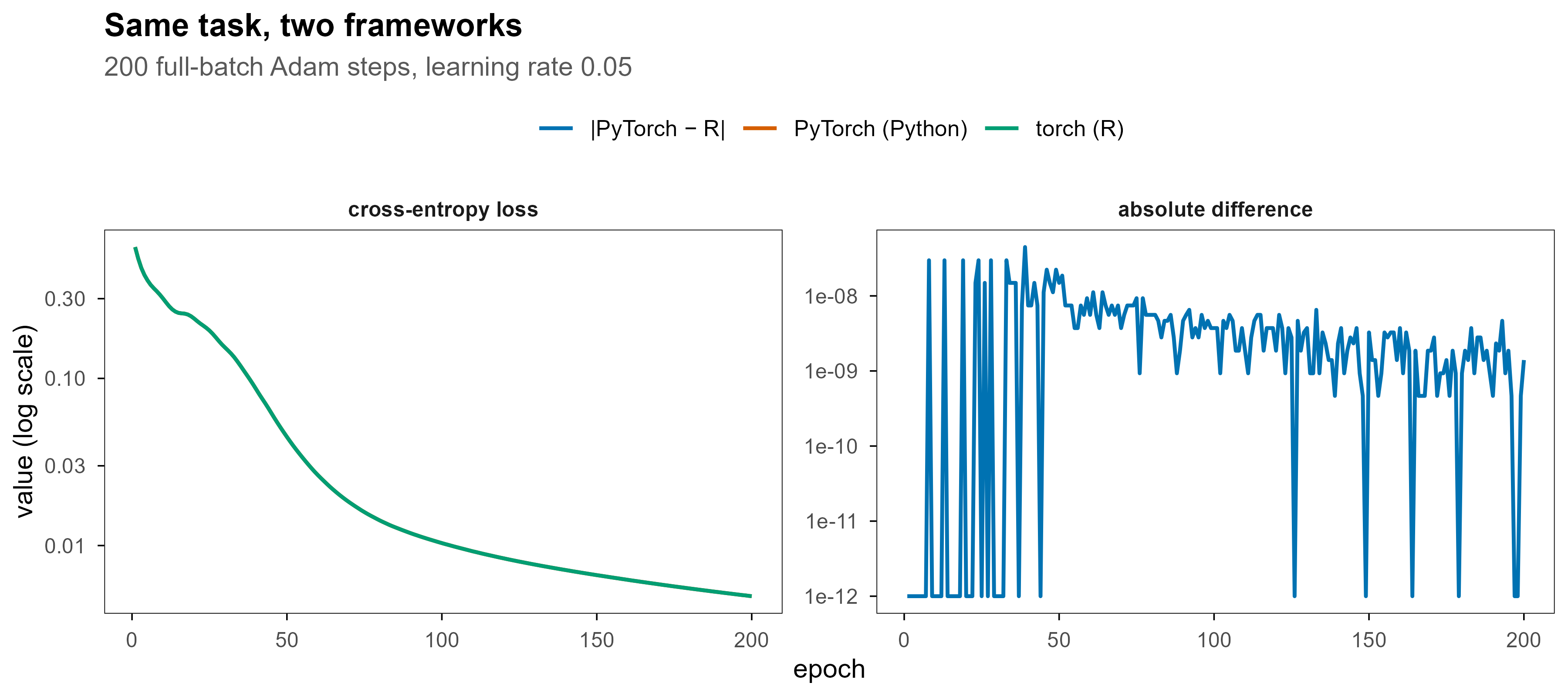
The training trajectories also almost coincide, which is more interesting than expected. The random number generator lives neither in R nor in Python but inside libtorch: torch_manual_seed(7) and torch.manual_seed(7) seed the same engine, and both models build their layers in the same order, so the initial weights are identical bit for bit. After 200 epochs the largest gap between the two loss sequences is 4.5e-08, purely a floating-point ordering artefact.
这个重合其实有点侥幸:两边的 libtorch 版本并不相同(R 侧 2.8.0,Python 侧 2.13.0),只是初始化与 Adam 在这两个版本之间的数值行为没有变。换个版本、换个建模顺序,或者中间插一个消耗随机数的算子,序列就会错开。所以被复现的是同一个引擎的状态,而不是”跨框架等价”。
The overlap is partly luck: the two libtorch builds are not the same (2.8.0 on the R side, 2.13.0 on the Python side); initialisation and Adam simply behave identically across these versions. A different build, a different construction order, or any random-consuming op in between would desynchronise the sequences. What is reproduced is the state of one engine, not a cross-framework equivalence.
8. 结果对比 / Comparing the results
Code
res <-data.frame(engine =c("PyTorch (Python)", "torch (R)"),version =c(py$ver_py, r_res$version),final =sprintf("%.4f", c(py$losses_py[[200]], r_res$losses[200])),accuracy =sprintf("%.3f", c(py$acc_py, r_res$acc)))kable(res,col.names =c("引擎 / Engine", "版本 / Version","末轮损失 / Final loss", "测试准确率 / Test acc"),caption ="同一数据、同一结构下的结果。 / Same data, same architecture.")
Table 1: 同一数据、同一结构下的结果。 / Same data, same architecture.
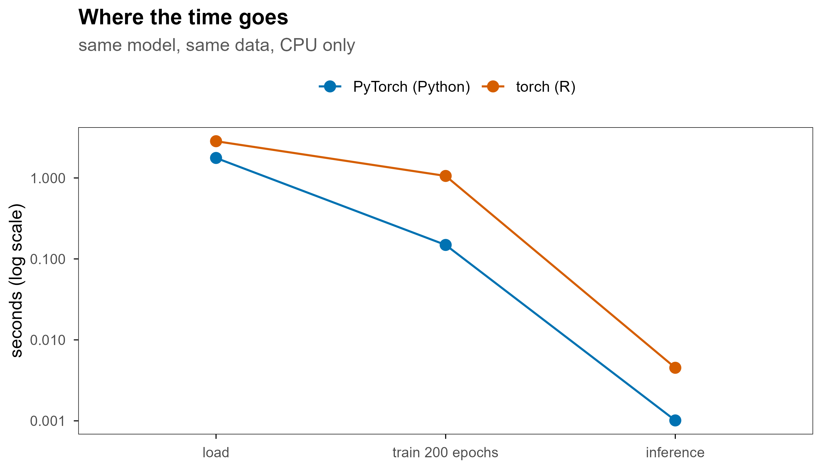
Both converge to near-zero loss within 200 epochs, and both reach 100% on the test split. At this scale the results are equivalent; everything that differs is time, and time splits into three parts.
Code
train_r <- r_res$secondstrain_py <- py$t_train_pytiming_tbl <-data.frame(engine =c("PyTorch (Python)", "torch (R)"),load =sprintf("%.2f", c(py$t_load_py, r_res$load)),epoch =sprintf("%.1f", 1000*c(train_py, train_r) /200),train =sprintf("%.2f", c(train_py, train_r)),infer =sprintf("%.1f", 1000*c(py$t_infer_py, r_res$infer)))kable(timing_tbl,col.names =c("引擎 / Engine", "加载 torch (s)", "每轮 (ms)","训练 200 轮 (s)", "网格推理 (ms)"),caption ="时间拆成三段:导入、训练、推理。加载只计 import / library 本身,不含解释器启动;推理前先各跑一次预热。 / Time in three parts: import, training, inference. Loading counts only import/library, not interpreter startup, and inference is measured after one warm-up pass.")
Table 2: 时间拆成三段:导入、训练、推理。加载只计 import / library 本身,不含解释器启动;推理前先各跑一次预热。 / Time in three parts: import, training, inference. Loading counts only import/library, not interpreter startup, and inference is measured after one warm-up pass.
引擎 / Engine
加载 torch (s)
每轮 (ms)
训练 200 轮 (s)
网格推理 (ms)
PyTorch (Python)
1.77
0.7
0.15
1.0
torch (R)
2.84
5.3
1.06
4.5
三段数字指向三种不同的东西。
The three segments point at three different things.
Loading is the same order of magnitude, 1.77 s versus 2.84 s; R is a little slower but not by an order of magnitude. Both have to map several hundred megabytes of libtorch into memory, so the cost is disk and dynamic linking rather than the language.
训练是唯一真正拉开差距的地方:R 每轮 5.3 ms,Python 每轮 0.7 ms,差 7.1 倍。R 的每一步都要跨一次 R 与 C++ 的边界,而 Python 的 autograd 与优化器都在 C++ 里跑完,只有一次 loss.item() 回到解释器。轮数越多、这个固定开销被摊得越薄;但每轮只有几毫秒时,接口成本占比就很可观。
Training is the only place where they really diverge: 5.3 ms per epoch in R against 0.7 ms in Python, a factor of 7.1. Every R step crosses the R/C++ boundary, whereas Python runs autograd and the optimiser entirely inside C++ and returns to the interpreter once, for loss.item(). The more epochs you run, the thinner that fixed overhead is spread; but when an epoch costs only a few milliseconds, the interface dominates.
Inference (6,400 points on an 80 × 80 grid) is in the millisecond range on both sides: 1.0 ms and 4.5 ms. The ratio is still a few-fold, but the absolute numbers are negligible — a forward pass was never the expensive part.
Code
timing <-data.frame(engine =rep(c("PyTorch (Python)", "torch (R)"), each =3),stage =factor(rep(c("load", "train 200 epochs", "inference"), 2),levels =c("load", "train 200 epochs", "inference")),seconds =c(py$t_load_py, train_py, py$t_infer_py, r_res$load, train_r, r_res$infer))ggplot(timing, aes(stage, seconds, colour = engine, group = engine)) +geom_line(linewidth =0.6) +geom_point(size =2.8) +scale_y_log10(labels = scales::label_number(accuracy =0.001)) +scale_colour_manual(values =c(blog_pal[["blue"]], blog_pal[["vermillion"]])) +labs(x =NULL, y ="seconds (log scale)", colour =NULL,title ="Where the time goes",subtitle ="same model, same data, CPU only")
Figure 2: 三个阶段的对数时间对比。加载与推理接近,训练差一个数量级。 | Log-scale comparison of the three stages. Loading and inference are close; training differs by an order of magnitude.
Figure 3: 左:两条损失曲线(对数纵轴),几乎完全重合;右:逐轮差值的绝对值,触到底线表示该轮两边完全相同。随机数生成器在 libtorch 里,两边播种的是同一个引擎。 | Left: two loss curves on a log axis, almost coincident; right: the per-epoch absolute difference, where the floor means the two runs agreed exactly. The RNG lives in libtorch and both sides seed the same engine.
Code
grid_flat <-as.matrix(expand.grid(x =as.numeric(py$gx), y =as.numeric(py$gy)))surf <-data.frame(x = grid_flat[, 1], y = grid_flat[, 2],py =factor(as.integer(py$Z_py)), r =factor(r_res$classes))surf_long <- tidyr::pivot_longer(surf, c(py, r), names_to ="engine", values_to ="class")surf_long$engine <-factor(surf_long$engine, levels =c("py", "r"),labels =c("PyTorch (Python)", "torch (R)"))ggplot() +geom_tile(data = surf_long, aes(x, y, fill = class), alpha =0.4) +geom_point(data = pts, aes(x, y, colour = class), size =1.1) +facet_wrap(~engine) +scale_fill_manual(values =c("0"="#CFE3F0", "1"="#F6D9C9"), guide ="none") +scale_colour_manual(values =c(blog_pal[["blue"]], blog_pal[["vermillion"]]),labels =c("class 0", "class 1")) +coord_equal() +labs(x =NULL, y =NULL, colour =NULL,title ="Where the two models put the boundary",subtitle ="shaded regions are predicted classes")
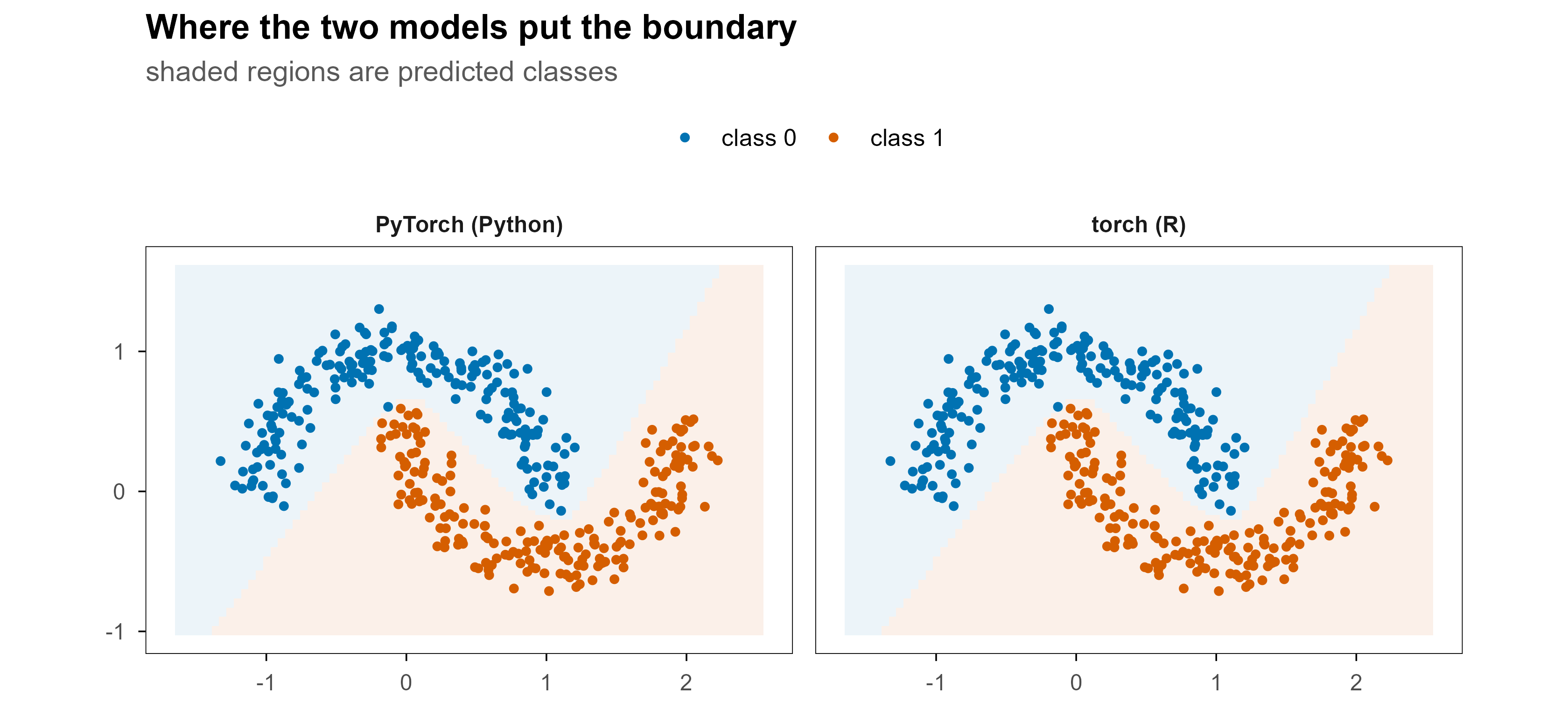
Figure 4: 决策面:左为 PyTorch,右为 R torch;点为真实类别。 | Decision surfaces: PyTorch left, R torch right; dots are the true classes.
The two surfaces are nearly identical: both boundaries fall between the half-moons, and the small differences near the edges come from different initial weights. On this task, the framework choice changes how the code feels to write, not what the model concludes.
9. 其他引擎的实测 / What the other engines did
9.1 Bash
{bash} chunk 在 Windows 上会去调用 bash,如果装了 WSL,实际执行的是 Linux 子系统。所以 uname 报的是 Linux,文件计数也是 Linux 侧看到的那个目录。
On Windows a {bash} chunk calls bash, which means WSL if installed, so uname reports Linux and the file count is whatever the Linux side sees in that directory.
Code
echo"shell: ${BASH_VERSION:-unknown}"uname-srprintf'qmd files in this folder: %s\n'"$(ls-1*.qmd 2>/dev/null |wc-l)"
shell: 5.2.37(1)-release
Linux 6.6.87.2-microsoft-standard-WSL2
qmd files in this folder: 1
9.2 OJS
OJS 是在浏览器里跑的,渲染阶段只会看到代码被嵌进 HTML。
OJS runs in the browser; at render time you only see the code being embedded into the HTML.
Code
vals = [1,2,3,4,5]total = vals.reduce((a, b) => a + b,0)"OJS says: sum = "+ total +", mean = "+ (total / vals.length).toFixed(2)
页面打开后上面这行字才会出现,它来自读者的浏览器,而不是构建机器。
That line only appears once the page is open, and it comes from the reader’s browser rather than from the build machine.
9.3 Julia
Julia 的代码看起来和 R、Python 的 chunk 一样自然,但这台机器上没有 Julia。下面这段现在只是一个普通代码块——原因见后文。
The Julia code looks as natural as an R or Python chunk, but this machine has no Julia. What follows is now an ordinary code block, and the reason is below.
knitr has to load JuliaCall when it registers the engine, which happens before eval is consulted. Turning execution off does not let a language without a runtime slip through; the only option is to demote it to a plain code block. This is probably the most useful conclusion in the post: eval: false will not save you.
10. freeze 与 code-fold 改变了什么 / What freeze and code-fold change
This site sets freeze: true in posts/_metadata.yml, so the numbers above are computed on the first render and then stored under _freeze/. Editing prose does not trigger recomputation; only changing a code chunk or deleting the matching _freeze directory does.
That has two consequences. First, the evidence that “it ran” can go stale: change the code while the cache survives, and readers still see the old output. Second, freeze is what makes a multi-language document practical, since a rebuild no longer has to start R, Python and bash every time.
code-fold: true affects presentation only, not execution: code is collapsed by default and expands on click. For a post whose point is the output, collapsing the code actually makes the results easier to read.
11. 结论 / Takeaways
两个框架都能跑,但坑不同。 Python 的 PyTorch 装好即用;R 的 torch 需要把 lib/ 目录加进 PATH,否则 lantern.dll 会报”找不到指定的过程”。 Both frameworks work, but they fail differently. PyTorch works out of the box; R’s torch needs its lib/ directory on PATH, or lantern.dll fails with “specified procedure could not be found”.
两个 libtorch 不能住进同一个进程。 想在 R 会话里用 reticulate 跑 PyTorch、同时又跑 R torch,必然有一方加载失败;只能分进程。 Two libtorch builds cannot share one process. Using reticulate to run PyTorch and R torch in the same session makes one of them fail to load; they have to be separated into processes.
一致性比想象中强。 同一个 exp().sum() 两边差 0.0e+00;连 200 轮训练曲线都几乎重合,因为随机数生成器和算子都在 libtorch 里,不在 R 或 Python 里。 Consistency is stronger than expected. The same exp().sum() differs by 0.0e+00, and even the 200-epoch loss curves nearly coincide, because both the RNG and the kernels live in libtorch rather than in R or Python.
时间差集中在训练轮内。 加载 torch 两边都在数秒之内(1.77 vs 2.84 秒),推理都是毫秒级;只有每轮训练 R 比 Python 慢 7.1 倍,因为每一步都要跨一次 R/C++ 边界。 The gap sits inside the training loop. Loading torch takes a few seconds on both sides (1.77 vs 2.84 s) and inference is milliseconds; only the per-epoch cost differs, with R slower by 7.1x because every step crosses the R/C++ boundary.
“能写 chunk”不等于”能执行 chunk”。{python}、{bash} 在渲染时执行,{ojs} 交给浏览器,{julia}、{sql} 取决于本机是否具备运行环境。 “Can write a chunk” is not “can execute a chunk”. {python} and {bash} run at render time; {ojs} is delegated to the browser; {julia} and {sql} depend on what the machine has installed.
freeze 是这类文档的前提,也是隐患。 它避免每次构建都重启多套运行时,但也让输出与代码可能不同步。 freeze is both the enabler and the risk: it avoids restarting several runtimes per build, but it lets output drift away from code.