Jie Hua’s Bioinformatics Notes
  • Archive
  • About

Home

A working notebook of reproducible bioinformatics — genomes, structures, and data visualization.

Bioinformatics Notes · Vol. 01

Jie Hua

Notes on bioinformatics, genomes, and the craft of data visualization.

Search the notes Ctrl K

Browse the archive

Since 2025 · Biomedical Center, LMU · Munich

Genomes Structures Viz

Latest notes

From the notebook

View all notes

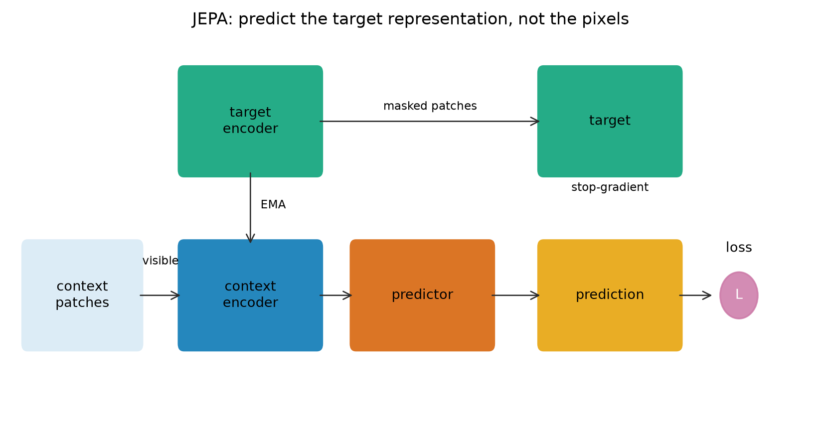
图 1 JEPA 的五个零件。上下文(可见 patch)经过上下文编码器;目标编码器(由 EMA 从上下文编码器缓慢复制而来)编码完整图像;预测器在目标位置填补 mask token 并输出预测;损失只作用在预测与”被 stop-gradient 挡住的目标”之间。 | Figure 1. The five parts of JEPA. Visible patches go through the context encoder; a target encoder (an EMA copy of the context encoder) encodes the full image; the predictor fills mask tokens at target positions; the loss compares the prediction with a stop-gradient target.

Predicting in Latent Space: An Anatomy of JEPA
从潜空间、自监督学习与表征坍塌这些基础概念讲起,拆开 JEPA 的目标函数、代码与十二张图,再落到 2022–2026 年的模型谱系与仍未解决的问题。
Jie Hua
Nov 18, 2026

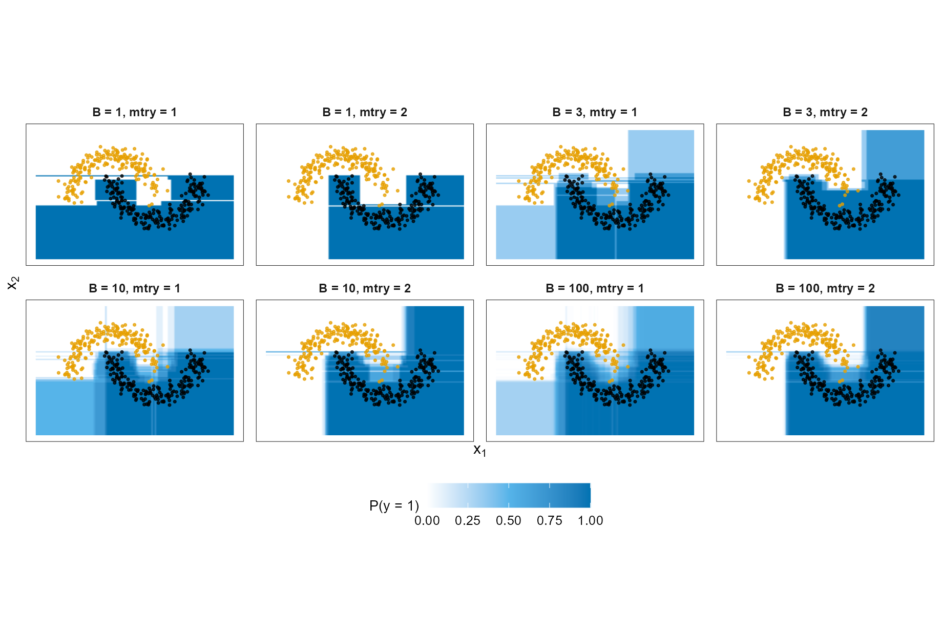
图 1 两个半月上的决策边界。B=1 时边界是几块矩形;B 增大后边界变细,但 mtry 决定它是否还能弯曲。训练误差很快归零,肉眼看到的差别主要是方差。 | Figure 1. Decision boundaries on two moons. At B=1 the boundary is a few rectangles; larger B refines it, while mtry decides whether it can still bend. Training error reaches zero quickly; most of the visible difference is variance.

The Correlation Floor: An Anatomy of Random Forests
从 AID 与 CART 到因果森林:用一次完整的消融实验拆开随机森林,推导并实测 ρσ²+(1−ρ)σ²/B,检验 OOB、解释性、校准、外推与成本,并给出今天的使用清单。
Jie Hua
Nov 18, 2026

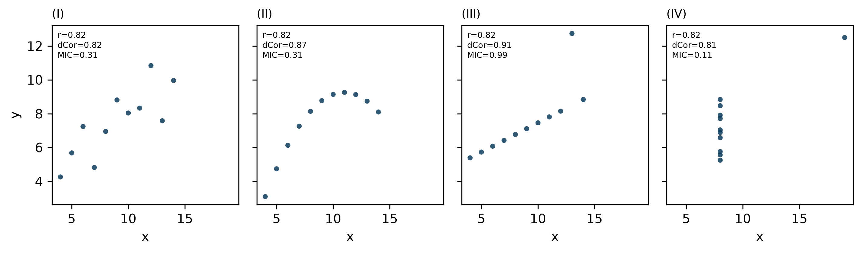
图 1 Anscombe 四组数据。四组的 Pearson r 都是 0.82;距离相关在 0.81–0.91 之间,而本文实现的 MIC 在 0.11–0.99 之间。注意 MIC 在 n = 11 时受 B(n) 限制,只能搜索很小的网格,数值不可跨样本量比较。 | Figure 1. Anscombe’s quartet. All four have Pearson r = 0.82; distance correlation ranges from 0.81 to 0.91, and the MIC implementation used here ranges from 0.11 to 0.99. Note that at n = 11 the B(n) bound restricts MIC to very small grids, so its values are not comparable across sample sizes.

Which Correlation? A Field Guide to Forty-Three Coefficients
把 43 个相关系数放到同一批数据上:零假设、不变性、置换校准、功效、异常值与计算成本,并给出选型表与误用清单。
Jie Hua
Nov 18, 2026

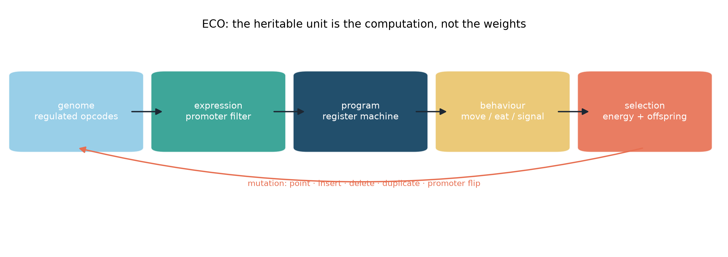
图 1 ECO 的结构:基因组 → 表达 → 程序 → 行为 → 选择,选择结果通过变异回到基因组。橙色箭头是唯一的”学习”通道,它不包含梯度。 | Figure 1. The ECO architecture: genome → expression → program → behaviour → selection, with the result of selection returning to the genome through mutation. The orange arrow is the only learning channel, and it contains no gradient.

What If We Never Invented Neural Networks?
如果计算的单位不是权重,而是可遗传的程序:一个约 300 行的寄存器机系统、20 个种子、五组消融,记录它能适应什么、不能适应什么。
Jie Hua
Nov 17, 2026

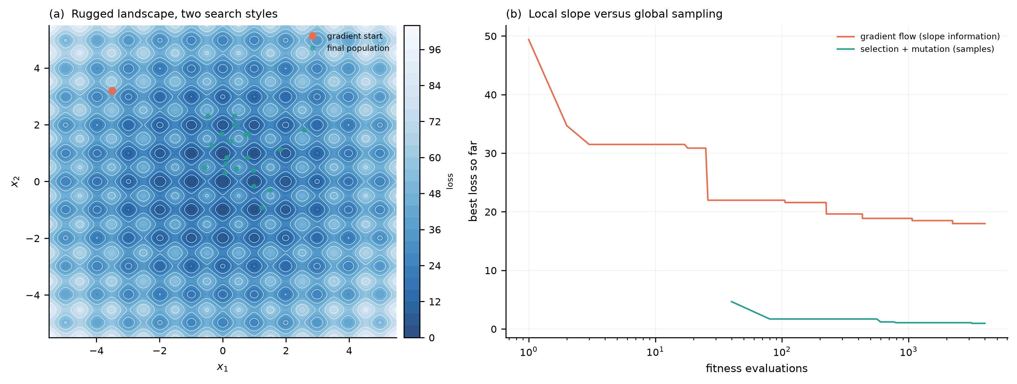
图 1 (a)Rastrigin 景观上的两种搜索:梯度流从一个点出发,选择维持一个种群。背景为损失等值线。(b)最优损失随评估次数的变化。梯度流困在局部极小(损失约 18),选择找到了接近全局的解(约 0.3)。 | Figure 1. (a) Two searches on the Rastrigin landscape: gradient flow starts from a single point, selection maintains a population. The background shows loss contours. (b) Best loss against evaluations. Gradient flow stalls in a local minimum (loss about 18) while selection finds a near-global solution (about 0.3).

Is Intelligence Evolved or Trained?
从细菌趋化到人工生态系统:四个可复现实验,比较梯度下降与自然选择、拓扑演化、质量—多样性搜索与分工的收益,并记录演化的失败条件。
Jie Hua
Nov 16, 2026

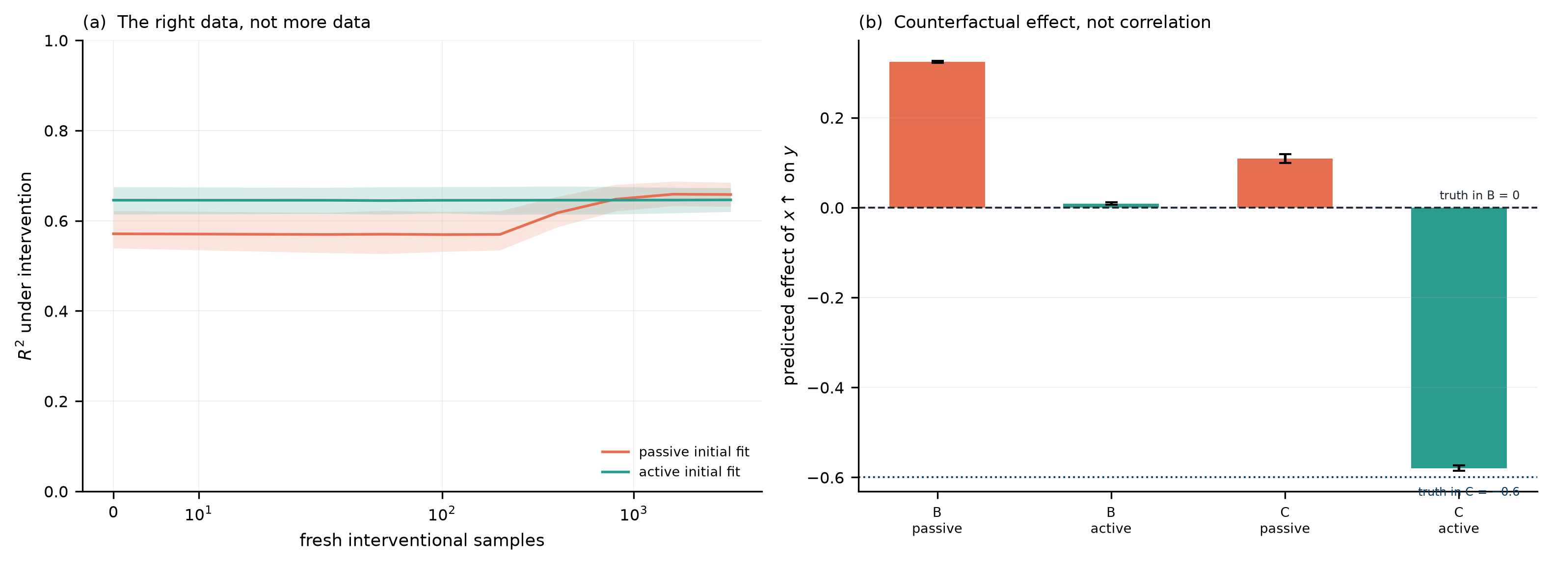
图 14 (a)被动学习器需要更多干预样本才能适应;主动学习器一开始就在正确的位置。(b)反事实效应估计:环境 B 的真值为 0,环境 C 的真值为 −0.6。被动学习器在 C 中给出 +0.11,符号错了。 | Figure 14. (a) The passive learner needs many more interventional samples to adapt; the active learner starts in the right place. (b) Counterfactual effect estimates: the true value is 0 in environment B and −0.6 in C. The passive learner gives +0.11 in C — the wrong sign.

Is the LLM the Final Road to AGI?
九个基准、四十条公开成绩与三组原创计算:LLM 的能力增长是否真的在放缓,Scaling Law 能推到哪一步,以及被动语料为何不足以识别因果结构。
Jie Hua
Nov 15, 2026

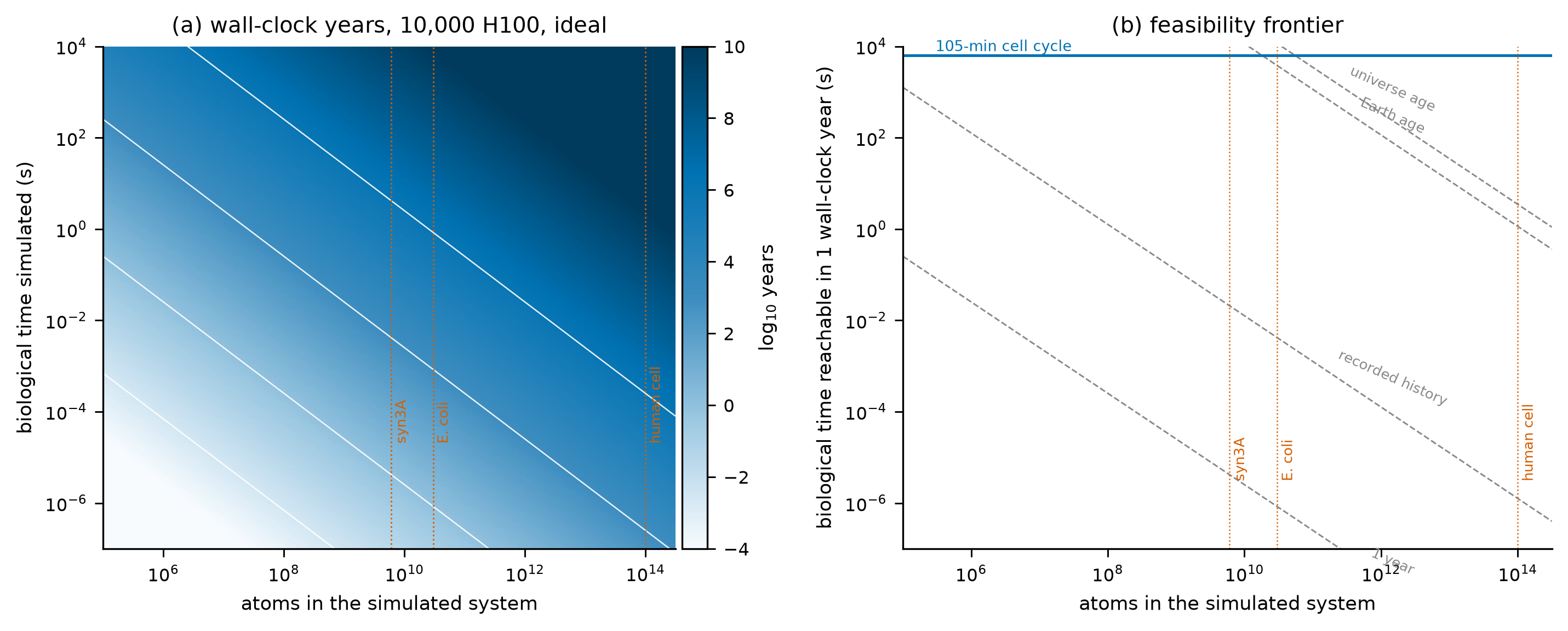
图 1 成本景观。(a) 在”一万块 H100、理想弱扩展”情景下,模拟不同原子数与不同生物时间所需的墙钟年数(对数色标);白线是 1 天、1 年、10³ 年、10⁶ 年的等值线。(b) 一年墙钟时间能触及的生物时间,作为原子数的函数;蓝线标出最小细胞的 105 分钟细胞周期。 | Figure 1. Cost landscape. (a) Wall-clock years needed to simulate a given atom count for a given biological time, under an ideal “10,000 H100” weak-scaling scenario (log colour scale); white contours mark one day, one year, 10³ and 10⁶ years. (b) Biological time reachable in one wall-clock year as a function of atom count; the blue line marks the 105-minute cell cycle of the minimal cell.

From Molecules to Cells: Can Microphysics Derive Life?
十组可复现计算,从全原子 MD 的成本墙、结构不可辨识性、Mori–Zwanzig 记忆,到非平衡通量、分岔、误差传播、空间与量子尺度。
Jie Hua
Nov 12, 2026
No matching items
Jie Hua Bioinformatics Notes
Archive About Homepage GitHub RSS
© 2025 · Built with Quarto · Published on Netlify